Magnet Model Project
Originally I only wanted to get some practice with the vector potential, magnetic and electric fields, and the resulting forces and torques. I thought I could do this by modeling magnets where I could put all the pieces together and also better understand how magnets work. I knew I was going to be making a lot of assumptions but I figured I could do someting relatively quickly to see if I was capturing the phsyics correctly.
This project quickly grew way beyond my original scope. Since the force goes as \(\frac{1}{r^3}\), I couldn't let the magnets get too close to each other since the equations would blow up. So I had to add some sort of constraint. I decided not to cut any corners with the collision constraint since the shape of the magnets was rectangular and somewhat simple to work with. I then decided to expand on this and introduce a collision response as well. These two pieces: collision detection and collision/impulse response actually took up most of the time I spent on the project.
So this project starts with covering the equations of motions, where they come from, and how I applied them to the rotating magnets utilizing rotating reference frames. The next two topics are the collision detection and impulse response parts of the model. I then give a better overview of the model and then compare the model to two simple magnet experiments. The layout of this project will be as follows (click the links to go to a specific section):
- Equations of Motion: Details on the equations of motion
- Rotating Frame:: Utilizing the quaternion to capture rotations
- Collision Detection: Details behind collision detection
- Impulse Response: Impulse response to represent the reaction to a collision
- Model Details and Example: Details on how the model is setup
- Model vs Experiment: Model results vs some simply magnet experiments
Equations
I will cover the basic equations I used to build the model and some details on their derivations. I relied heavily on Feynman's Lectures on Physics Volume 2 for this part of the project and refer the reader to him for the details on where the equations come from. I also won't show the derivation of the vector potential or exactly what it means. The vector potential is very useful here because it already combines the interactions between the electric and magnetic fields so we can find forces and torques almost directly from the vector potential. The vector potential is:
$$ \bar{A}(1) = \frac{1}{4 \pi \epsilon_o c^2} \int{\frac{\bar{j}(2)dV_2}{r_{12}}} $$where we are finding the vector potential at location 1 due to flowing charges at location 2. Feynman uses an analogy between the electrostatic potential and the magnetic dipole to solve this equation for the magnetic dipole. I wanted to try finding this using the equations and simplifying the integration. My method is as follows:
We start with a diagram of the magnetic dipole
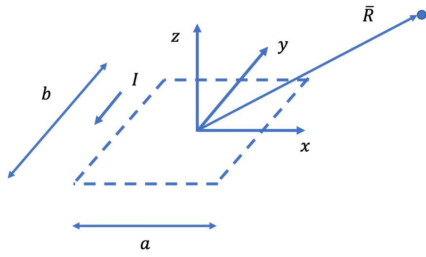
We have the current following the dotted box in the counter clockwise direction. We are interested in finding the vector potential at the location \(\bar{R}\). We first focus on finding the y-component of the vector potential so we have:
$$ A_y = \frac{1}{4 \pi \epsilon_o c^2} \int{\frac{j_y dV_2}{r_{12}}} $$We also have that \(I_y = j_y S\) and our current is flowing in a straight line so we integrate along y:
$$ A_y = \frac{I}{4 \pi \epsilon_o c^2} \int{\frac{dy}{r_{12}}} $$We have two segments so we have:
$$ A_y = \frac{I}{4 \pi \epsilon_o c^2} ( \int_{seg 1}{\frac{dy}{r_{12}}} - \int_{seg 2}{\frac{dy}{r_{12}}} )$$Note the direction of the current and the signs. Segment 1 refers to the segment where the current is in the positive y direction. In finding the vector potential, there is an assumption that we are looking at the potential at a large distance relative to the dimensions of the magnetic dipole. If we follow this to the extreme then we have:
$$ A_y \approx \frac{\partial A_{y,o}}{\partial x}dx = \frac{\partial A_{y,o}}{\partial x}a $$So we then want to find the vector potential at the origin from a segment of current flowing in the positive y direction. To find this, we can re-orient our figure so that we have a plane that includes the y axis and the point \(\bar{R}\). This is shown in the figure below:
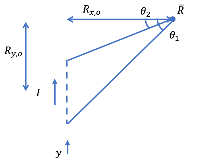
We have then:
$$ A_{y,o} = \frac{I}{4 \pi \epsilon_o c^2} \int{\frac{dy}{r}} $$Where we then have:
$$ y = R_{y,o} - r \sin\theta $$ $$ dy = -\sin\theta \, dr - r \cos\theta \, d\theta $$ $$ R_{x,o} = r \cos\theta $$ $$ dr = \tan\theta \, d\theta $$We can then use this to find \(\int{\frac{dy}{r}}\):
$$ \int{\frac{dy}{r}} = - \int_{\theta_1}^{\theta_2}{(\sin\theta\tan\theta + \cos\theta)} d\theta $$ $$ = -\ln(\tan\theta+\cos\theta) |_{\theta_1}^{\theta_2} = -\ln(\frac{y+r}{x}) |_{\theta_1}^{\theta_2}$$The natural log is nonlinear but we can get around this by saying we are looking at the integral over a small region where the function is approximately linear so we can take the Taylor series approximation:
$$ = -\ln(\frac{y+r}{x}) |_{\theta_1}^{\theta_2} \approx -[\ln(\frac{y_o+r_o}{x_o}) + \frac{1}{\frac{y_o+r_o}{x_o}}\frac{1+\frac{\partial r}{\partial y}}{x_o} dy] |_{-\frac{b}{2}}^{\frac{b}{2}}$$ $$ = -\frac{b}{r_o} = -\frac{b}{|\bar{R}|} $$We then have:
$$ A_{y,o} = - \frac{I}{4 \pi \epsilon_o c^2} \frac{b}{|\bar{R}|} $$ $$ A_y \approx \frac{\partial A_{y,o}}{\partial x} a = \frac{Iab}{4 \pi \epsilon_o c^2} \frac{x}{|R|^3} $$We have something similar for \(A_x\) but we have to be careful. For \(A_x\), we have in our approximation:
$$ A_x \approx -\frac{\partial A_{x,o}}{\partial y}dy = -\frac{\partial A_{x,o}}{\partial y}b $$The negative sign is because of the direction of the current and the direction of the magnetic moment. We then have:
$$ A_x \approx -\frac{Iab}{4 \pi \epsilon_o c^2} \frac{y}{|R|^3} $$We then use the same reasoning as Feynman and find the vector potential from a magnetic dipole as:
$$ \bar{A} = \frac{1}{4 \pi \epsilon_o c^2} \frac{\bar{\mu} \times \bar{R}}{R^3} $$We now have the vector potential and can use this with our magnetic dipole, \(\bar{\mu}\), to find the forces and moments on each magnet from the other. We will neglect gravity and other body forces. The magnetic dipole strength will be found experimentally. For the forces and moments, we wil use the following:
$$ \bar{F} = \nabla (\bar{\mu} \cdot \bar{B}) $$ $$ \bar{T} = \bar{\mu} \times \bar{B} $$ $$ \bar{B} = \nabla \times \bar{A} $$Feynman explains where the first two equations come from well. Basically the argument for the first equation is that work is defined as \(work=-\int F \cdot ds\) and for the case with a magnetic dipole in an external field (in our situation, one magnetic dipole represents one magnet and the other magnet produces the magnetic field), you can say \(F=\nabla(\bar{\mu} \cdot \bar{B})\). There are work sources that are neglected such as the work needed to sustain the magnetic field but those sources are neglected and what is left is called virtual work. You can also make the argument that the energy from the torque is \(dU=\bar{T} \cdot \bar{d \theta}\) which then gives (assuming torque and \(\theta\) are in the same direction) \(dU=-|\bar{\mu}||\bar{B}|cos(\theta)+C=-\bar{\mu}\cdot\bar{B} + C\). Then use have \(work=-\int F \cdot ds\) and you can say \(F=\nabla (\bar{\mu}\cdot\bar{B})\). The way I interpret this argument is that a magnetic moment in a magnetic field stores energy and you can say that some force was needed to put the magnetic moment in that orientation in the field. That then represents the work you need to put in the system.
The second equation (torque) might be a little easier to understand. Assuming again that a small current around a rectangular area is the magnetic dipole sitting in an external force, you can use \(F=q(\bar{E} + \bar{V} \times \bar{B})\) to find forces on each side of the dipole which create a torque balance on the dipole that can be represented by \(\bar{T} = \bar{\mu} \times \bar{B}\).
The third equation, the magnetic field, comes from our understanding of no magnetic charges so we have \(\nabla \cdot \bar{B} = 0\) which means that \(\bar{B}\) is the curl of something since the divergence of curl is always 0. This is part of the reasoning for the derivation behind what the vector potential is. Since our forces and torques are found from the magnetic field, it is nice to be able to find the magnetic field directly from the vector potential.
We first find the magnetic field and then we find the force. We can find the torque directly after we find the magnetic field. I won't show the details of the derivations (it is not exactly difficult but it can be a little messy). The magnetic field is (note I am using \(\bar{r}\) instead of \(\bar{R}\) now):
$$ \bar{B} = \frac{1}{4 \pi \epsilon_o c^2 r^5} [3(\bar{\mu} \cdot \bar{r})\bar{r} - \bar{\mu}r^2] $$When looking at the force equation, we are finding the force on magnet 1 from magnet 2 so in our equation, we have \(\bar{F}_{12} =\nabla (\bar{\mu}_1 \cdot \bar{B}_2)\) where the force is on magnet 1 and the magnetic field is from magnet 2. The force is then generally found as:
$$ \bar{F}_{ij} = \frac{3}{4 \pi \epsilon_o c^2 r^4}[(\bar{\mu}_i\cdot\bar{r}_{ij})\bar{\mu}_j + (\bar{\mu}_j\cdot\bar{r}_{ij})\bar{\mu}_i + (\bar{\mu}_i\cdot\bar{\mu}_j)\bar{r}_{ij} - 5(\bar{\mu}_i\cdot\bar{r}_{ij})(\bar{\mu}_j\cdot\bar{r}_{ij})\bar{r}_{ij}] $$We find that the forces are equal and opposite for each magnet which makes sense since we understand each force has an equal and opposite reaction. Finding the torque is straightforward using the cross product. The nice part of using the vector potential is that we don't have to worry about how the changing magnetic and electric fields interact with each other, this is already baked in to the vector potential.
We don't have to work out the torque equation in detail like we did the force equation. This is because we can directly find the cross product. Finding the gradient is a little more involved so we did out the equation and will implement in this code later. Also note that we can see how the single magnetic momemnt approximation breaks down. Fields are linear, we can add the field from one magnetic moment and from another. We can also do the same for the force. The problem is the force goes to \(\frac{1}{r^3}\) and at small distances this can lead to very different forces depending on the distance so if we represent the magnet as many different magnetic moments (which I'm guessing is how real simulation tools work), we would have much different forces when the magnets are close to each other if we have a single magnetic moment or multiple. The magnetic field also goes as \(\frac{1}{r^3}\) so we have the same issue with multiple magnetic fields from multiple magnetic moments. If we have multiple magnetic moments, we also now capture more torques on the magnets.
At the end of this project, we will compare the result from the model to a magnet experiment. If the magnetic moment is weak enough and the magnet is large enough, the distances (due to the magnets not being able to penetrate each other) may be sufficient for the single magnetic moment approximation to be somewhat valid.
Rotating Frame
We can now find our equations of motion and put these in a form that is most suitable for us. We have:
$$ \bar{F} = m \frac{d\bar{V}}{dt} $$ $$ \bar{T} = \frac{d (I \times \bar{\omega})}{dt} = \frac{d\bar{H}}{dt} $$In the above, \(m\) is our mass, \(\bar{V}\) is our velocity, \(I\) is our moment of inertial (matrix), and \(\omega\) is our angular velocity. We also have \(\bar{H}=I \times \bar{\omega}\). Since our magnets are rotating, it is best to expand our force and torque equations (that are expressed in the inertial frame) to use the body or rotating reference frame values:
$$ \bar{F} = (m\frac{d\bar{V}}{dt})_b + m \bar{\omega} \times \bar{V}_b $$ $$ \bar{T} = (\frac{d\bar{H}}{dt})_b + \bar{\omega} \times \bar{H}_b $$ $$ \bar{T} = (\frac{d (I \times \bar{\omega})}{dt})_b + \bar{\omega} \times I_b \times \bar{\omega} $$The \(\omega\) cross product term comes from the rotation. Basically we have in the general case \(\frac{d}{dt}\bar{f_i}=\frac{d}{dt}\bar{f_b}=\frac{d}{dt}(f_{b,x}\hat{i_b},f_{b,y}\hat{j_b},f_{b,z}\hat{k_b})\). Expanding the derivative gives \(\frac{d}{dt}\bar{f_b}=(\frac{df_{b,x}}{dt}\hat{i_b},\frac{f_{b,y}}{dt}\hat{j_b},\frac{f_{b,z}}{dt}\hat{k_b})+(f_{b,x}\frac{d\hat{i_b}}{dt},f_{b,y}\frac{\hat{j_b}}{dt},f_{b,z}\frac{d\hat{k_b}}{dt})=\frac{d\bar{f_b}}{dt}=\bar{\omega}\times\bar{f_b}\). It's easiest to understand and work this out in the 2D case and generalize to the 3D case. Subscript \(b\) denotes body frame compared to inertial frame. We find the forces and torques in the inertial frame (non-rotating frame) but we use the velocities and moment of inertia in the rotating frame. Since we are not considering any deformities, our moment of inertia matrix stays constant.
It's clear we need a method to go back and forth between the rotating and non-rotating frames. We will use the quaternion to do this. We could also use rotational matrices but this can lead to instabilities at certain angles and the quaternion is more robust to this. We’re not going to show how the quaternion gives a rotation, there are other good references that summarize that and it can be a time consuming exercise to do. I recommend looking at this summary: Quaternions And Dynamics by Basile Graf (Arxiv link). The quaternion is:
$$ q = (q_0 , q_1 , q_2 , q_3) = q_0 + q_1i + q_2j + q_3k $$where \(q_0\) is usually denoted as the real part and the rest is the imaginary. We sometimes see:
$$ q = (q_0,\bar{q}) $$where \(\bar{q}=(q_1,q_2,q_3)\) is the vector part. The conjugate of the quaternion is:
$$ q' = (q_0,-\bar{q}) $$Quaternion multiplication follows:
$$ ii = jj = kk = ijk = -1 $$So we get:
$$ qp = (q_0,\bar{q})(p_0,\bar{p}) = (q_0p_0-\bar{q}\cdot\bar{p},q_0\bar{p}+p_0\bar{q}+\bar{q}\times\bar{p}) $$Rotations using the quaternion follow (this is where the reference I gave above gives a good description. It can be involved so I'm not going to repeat it here. There are other good sources out there as well):
$$ (0,\bar{f_i}) = q(0,\bar{f_b})q' $$The vector we are interested in is \(\bar{f}\) where we want to translate from the body frame to the inertial frame. There is no real part when you take a physical vector and make a quaternion. We then can also say:
$$ \bar{f_i} = R\bar{f_b} $$Skipping the details, you can then show (after expanding the quanternion):
$$ R = \begin{bmatrix} q_0^2+q_1^2-q_2^2-q_3^2 & 2(q_1q_2-q_0q_3) & 2(q_1q_3+q_0q_2) \\ 2(q_2q_1+q_0q_3) & q_0^2+q_2^2-q_1^2-q_3^2 & 2(q_2q_3-q_0q_1) \\ 2(q_1q_3-q_0q_2) & 2(q_2q-3+q_0q_1) & q_0^2+2_3^2-q_1^2-q_2^2 \end{bmatrix} $$Using the above, we can translate between the quaternion and the corresponding rotation matrix. This will come in handy when we are plotting and troubleshooting. We can also show how if you can define two axis vectors in both frames (inertial or body/rotating), it is easy to build the rotation matrix and then get the quaternion. One can use:
$$ R_i = R R_b $$ $$ R_i = (x_i, y_i, z_i) $$ $$ R_b = (x_b, y_b, z_b) $$With two axis vectors in one frame, we can find a third that is perpendicular to both. You can then build the \(R_i\) and \(R_b\) matrices and then find \(R=R_iR_b^{-1}\).
The next tricky part of the quaternion is finding the quaternion time derivative. As we are stepping throught time, the rotation is changing the orientation of each magnet and we need to keep track of this orientation using the quaternion so we are interested in finding the quaternion time rate of change. The reference I linked above starts the derivation assuming there is a fixed vector in the body frame. I wanted to see if I could get the same answer with the opposite starting point, starting with a fixed vector in the inertial frame. The derivation starts with:
$$ x_i = qx_bq' $$ $$ x_b = q'x_iq $$In the above, superscript \('\) denotes the conjugate. We are interested in the quaternion which translates from body to inertial. We can take the time derivative of the second equation and get:
$$ \dot{x}_b = \dot{q}'x_iq + q'x_i\dot{q} $$We are assuming that \(x_i\) is fixed. We can plug in our original equation for \(x_i\):
$$ \dot{x}_b = \dot{q}'qx_bq'q + q'qx_bq'\dot{q} = \dot{q}'qx_b + x_bq'\dot{q} $$ $$ \dot{q}'q = (\dot{q}_0q_0 + \dot{q}_1q_1 + \dot{q}_2q_2 + \dot{q}_3q_3, \dot{q}_0\bar{q} + q_0\dot{\bar{q}}' + \dot{\bar{q}}' \times \bar{q}) = (0, \dot{q}_0\bar{q} + q_0\dot{\bar{q}}' + \dot{\bar{q}}' \times \bar{q}) $$ $$ q'\dot{q} = (\dot{q}_0q_0 + \dot{q}_1q_1 + \dot{q}_2q_2 + \dot{q}_3q_3, -(\dot{q}_0\bar{q} + q_0\dot{\bar{q}}' + \dot{\bar{q}}' \times \bar{q})) = (0, -(\dot{q}_0\bar{q} + q_0\dot{\bar{q}}' + \dot{\bar{q}}' \times \bar{q})) $$ $$ \dot{q}_0q_0 + \dot{q}_1q_1 + \dot{q}_2q_2 + \dot{q}_3q_3 = \frac{1}{2}\frac{d}{dt}|q^2| = \frac{1}{2}\frac{d}{dt}(1) = 0 $$The quaternion's magnitude is always 1 so that's where the last expression comes from. We can also say:
$$ \dot{q}'q = (0, \dot{q}_0\bar{q} + q_0\dot{\bar{q}}' + \dot{\bar{q}}' \times \bar{q}) = (0,\bar{v}) $$ $$ q'\dot{q} = (0, -(\dot{q}_0\bar{q} + q_0\dot{\bar{q}}' + \dot{\bar{q}}' \times \bar{q})) = (0,-\bar{v}) $$So then we have:
$$ \dot{x}_b = \dot{q}'x_iq + q'x_i\dot{q} = (0,\bar{v})x_b + x_b(0,-\bar{v}) $$ $$ (0,\dot{x}_b) = (0,\bar{v})x_b - x_b(0,\bar{v}) = (-\bar{v}\cdot\bar{x}_b,\bar{v}\times\bar{x}_b) - (-\bar{x}_b\cdot\bar{v},\bar{x}_b\times\bar{v}) $$ $$ \dot{\bar{x}}_b = 2\bar{v}\times\bar{x}_b = \bar{\omega}_b\times\bar{x}_b $$The last expression comes from understanding that the rate of change of our vector is perpendicular to the vector. We understand this as a rotation. However, we need to be careful about our understanding of what rotation we are talking about. Remember we had assumed that the vector in the inertial frame is not changing so when the rotating frame is rotating, the vector \(\bar{\omega}_b\) is rotating in the opposite direction compared to the direction the frame is rotating in. Hopefully you can visualize this in the schematic below.
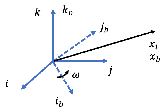
Imagine the rotating frame rotating counter clockwise around the z axis. The rotating frame is rotating with respect to the inertial frame. In the inertial frame, the vector \(x_i\) is constant (e.g., not moving). However, in the rotating frame, the vector \(x_b\) would be seen to be rotating clockwise. The clockwise rotation is what \(\bar{\omega}_b\) is in the above equation. We are interested in the rotation with respect to the inertial frame so that is \(\bar{\omega} = -\bar{\omega}_b\).
We then have:
$$ \dot{\bar{x}}_b = 2\bar{v}\times\bar{x}_b = \omega_b\times\bar{x}_b = -\bar{\omega}\times\bar{x}_b $$ $$ \bar{v} = -\frac{1}{2} \bar{\omega} $$which gives:
$$ q'\dot{q} = (0,-\bar{v}) = \frac{1}{2}(0,\bar{\omega}) $$ $$ \dot{q} = \frac{1}{2}q(0,\bar{\omega}) $$We can do this out to get something easier to implement in the code:
$$ \dot{q} = \frac{1}{2} \Omega \times q $$ $$ \Omega = \begin{bmatrix} 0 & -\omega_x & -\omega_y & -\omega_z \\ \omega_x & 0 & \omega_z & \omega_y \\ \omega_y & -\omega_z & 0 & \omega_x \\ \omega_z & \omega_y & -\omega_x & 0 \end{bmatrix} $$So to recap we found how to express our equations of motion using the rotating frame as a reference. We can calculate our forces and torques in the inertial frame and find our translational accelerations and angular accelerations in the rotating frame as well as our quaternion rate of change. We use this to find our translational and angular velocities in the rotating frame using a numerical solver. We then can use the quaternion to find the inertial frame velocities and integrate. This is a high level summary of how we will implement what we just learned.
Collision Detection
At first I was planning on ignoring collision detection since I just wanted to get a feel for how the magnets would interact with eachother. However, since \(F \propto \frac{1}{r^3}\), my velocities get very large when the dipoles get close and my model blows up. So I needed a way to restrict movement. I could have done this in an easier way but I figured I could capture the physics as best I could. This section will discuss the basics behind collision detection and the next section discusses how I have the magnets respond once a collision is detected.
Our approach is based on the Separate Axis Theorem which is based on the theorem that if two non-empty convex subsets, A and B, are non-intersecting then:
$$ (x \cdot v) \le c \, and \, (y \cdot v) \ge c $$ $$ for \, all \, x \in A \, and \, y \in B $$where \(v\) is the unit normal in the direction separating A and B, \(x\) and \(y\) are vectors, and \(c\) is a constant scalar. A schematic of the theorem is shown below:
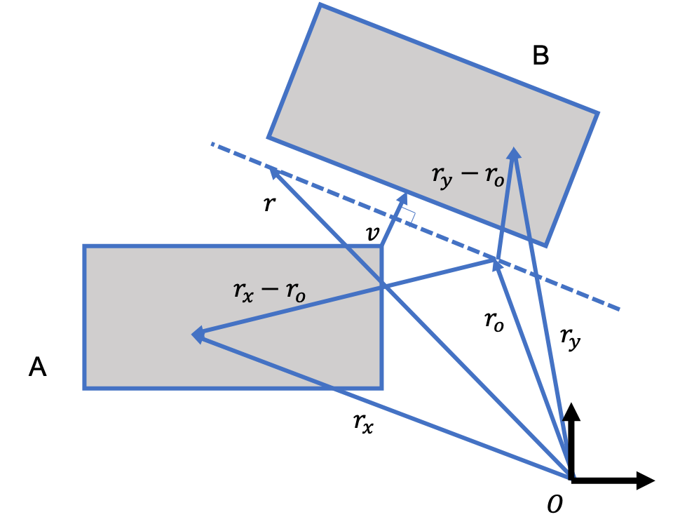
Looking at the schematic, we note that A and B are separate. \(v\) is the normal in the direction seperating A and B and points from A to B. We know that the equation of a plane (or a line in the 2D case) is:
$$ (r-r_o) \cdot v = 0 $$Looking at \(r_x\), we then have:
$$ (r_x - r_o) \cdot v = l < 0 $$Looking at the geometry, we know that \(\theta\) is always greater than 90 degrees and/or less than -90 degrees which makes the dot product less than 0. We also have:
$$ (r_y - r_o) \cdot v = m > 0 $$Looking at the geometry again, we know that \(\theta\) is always between -90 and 90 degrees so the dot product is greater than 0.
We can then say that \(r_o \cdot v = c\) and then we have:
$$ r_x \cdot v \le r_o \cdot v = c $$ $$ r_y \cdot v \ge r_o \cdot v = c $$Which is what the theorem says. This also extends to the 3D case which is what our magnet model will be.
Our collision detection method is based off this theorem. We can start with the simpler 2D case. If we have two non-overlapping rectangles, it's not hard to visualize that the seperating line must be parallel to one of the rectangles edges. For the 2D case with rectangles, we then have 4 directions to test corresponding to the two axes of each rectangle. This can be seen in the figure below where the seperating line is perpendicular to the \(y_B\) direction.
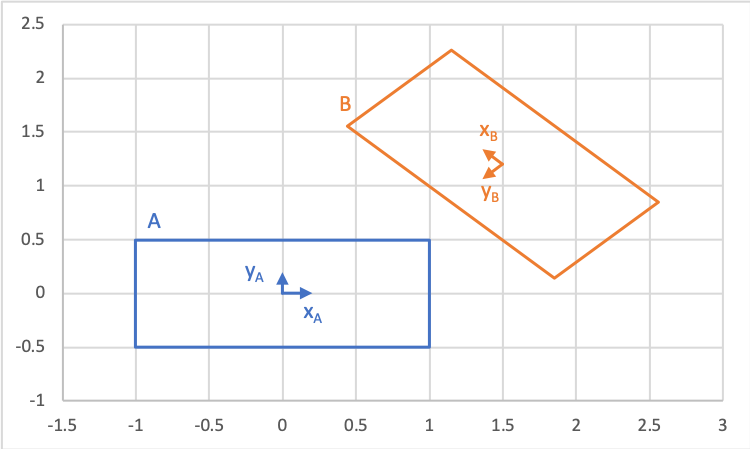
We need to check along each direction (4 directions total for the 2D case, 15 total for the 3D case) and check for collision. We only need to find one direction that doesn't produce a collision. So for each direction, we have a vector which we still denote as \(v\). We also have a vector that goes from the center of one block to the center of the other. We denote this by \(T\). At this point, the direction of \(v\) and \(T\) doesn't matter. We then want to compare the sum of projection of each block in this direction to the projection of \(T\) in this direction. If the sum of the block projections is greater than the center to center projection, then we have an overlap which means collision in that direction. If it is the opposite, we have no collision in that direction and thus no collision at all since we can draw a line that seperates the blocks (see the figure below and above).
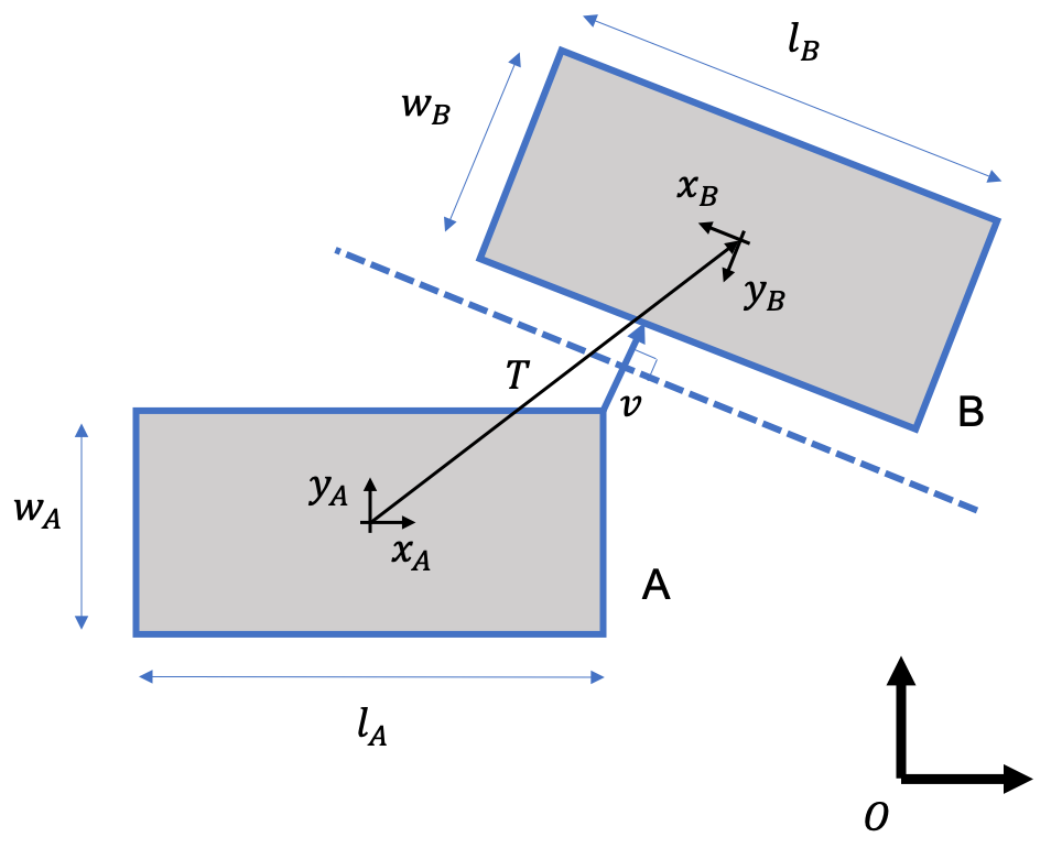
To illustrate the algorithm, we have four directions to test: \(x_A,y_A,x_B,y_B\). We can represent the direction by \(n\). For the block projection, we don't really care about the direction since we are ultimately comparing two scalars so we have:
$$ Block \, Projection \, Sum = \sum_A |e_A \cdot n | \frac{d_A}{2} + \sum_B |e_B \cdot n | \frac{d_B}{2} $$ $$ = |x_A \cdot n| \frac{l_A}{2} + |y_A \cdot n| \frac{w_A}{2} + |x_B \cdot n| \frac{l_B}{2} + |y_B \cdot n| \frac{w_B}{2} $$ $$ Center-to-Center \, Vector \, Projection \, Sum = |T \cdot n| $$If the Block Projection Sum is greater than the Center-to-Center Vector Projection Sum, then we have a collision in that direction. If the Center-to-Center Vector Projection Sum is greater than the Block Projection Sum then we have no collision in that direction and no collision at all. We only need one direction to pass the collision test to say there is no collision. The schematic below shows what distances are calculated in the alogrithm so you can better understand what is happening.
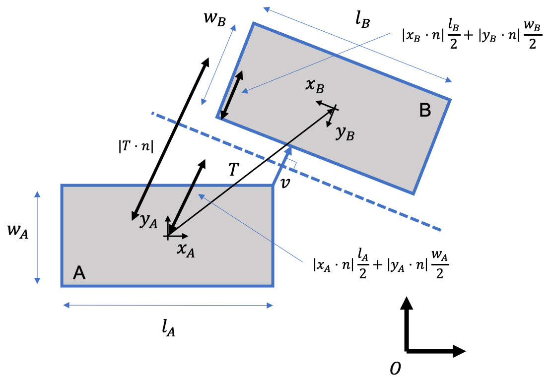
We see how for each direction, \(\sum |e_i \cdot n| \frac{d_i}{2} \) is fixed for each block. As we move the blocks closer together, \(|T \cdot n|\) becomes smaller and eventually the block projection will be greater than the center-to-center vector projection and we conclude a collision.
In the 2D case, we only need to check 4 directions. In the 3D case, we have 15 directions. 3 are for one magnet (block) and 3 more are for the second. The other 9 directions come from the cross products of the 3 for block A and 3 for block B.
It's fairly intuitive to understand why we need to check the 3 axes of magnet A and the 3 axes of magnet B. The cross product directions are a little more difficult to understand. We will illustrate through this an example. The scenario where you need to check the cross product directions is the edge-edge case where the closest parts of each magnet to each other are part of the edges. The first 6 axes may fail to find edge-edge seperation. A face-edge seperation will be found using the first 6 axes as well as face-face which is a little more obvious. In the 2D case, we can only have face-face or face-edge so no need for cross products.
In our example, we will show how the face-face checks (the 3 axes of each magnet so 6 axes in total). We will also show that the vector representing the smallest distance between each block is perpendicular to at least one axis of each magnet. This is part of the reason we need to check those axes.
We choose how to rotate our blocks in this example. One block we leave alone and don't rotate and the other rotate so that when looking at the shortest distance between the two blocks, we have two points with one on an edge of each block. The blocks are shown in the figures below (it can be difficult to visualize so I suggest running the code yourself to see the blocks better and rotate them):
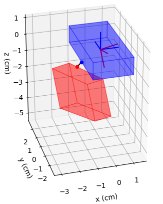
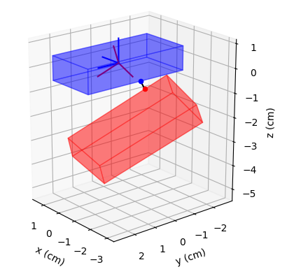
It may take some studying but we can visualize how looking at the axes of each block doesn't give separation of the blocks. However, we see that the blocks are clearly separated. We see that for each main axis of each block, when we project each block against that direction, we have the addition of each projection (taking the absolute value of the projection since the blocks are symmetric) being larger than the absolute value of the projection of vector separating the blocks on that direction.
As an example, let's consider the z direction of the blue box. This is shown in the schematic below:
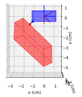
We see that if we take the sum of the absolute value of the projection of the red block's axes against the z direction and the absolute value of the projection of the blue block against the z direction, that we will have a larger number than the absolute value of the projection of the vector seperating the two block centers against the z direction. This is seen in the red block extending past the blue block. The sum of the projections of the red block against the z direction (really it's half of the projection since the block is symmetric, we are looking at projecting half the block from the center on to our axis), represents the distance along the z axis from the center of the red block to the tip of the red block. We see that this distance clearly intersects the blue block and therefore, no separation is found along this axis.
We can repeat the above for the other 5 axes (2 more from the blue block, 3 from the red) and reach the same conclusion. Clearly, the blocks don't intersect and this means we need to consider the cross products of the axes giving another 9 directions.
In our example, we have an edge-edge case where the closest points separating the two blocks fall on the blocks edges. This is represented by the black line connecting each edge. We also know that the black line (or vector) is perpendicular to at least one axis of each block. The edge essentially represents a vector in the direction of one of the block's main axes. From geometry, we know that the vector representing the smallest distance from a point to another vector is perpendicular to the latter vector. Since, we can make the same argument about each point, the vector representing the smallest distance between each block is perpendicular to each edge (and each edge represents one of the block's main axes). In this example, the two axes are the blue block's y axis and the red block's body frame y axis. The red block is rotated so it's body frame y axis doesn't point in the inertial frame y axis. If we take our sum of the absolute values of the projection of each block on the cross product of those two y axis directions, we find separation.
This topic took some time for me to fully appreciate it and I hope I can at least somewhat convey the idea here. It is helpful to write the equations down and look at an example.
Impulse Response
When a collision is detected, we need a method for how the magnets should response. This is the motivation for this section. When a collision is detected, we iterate until we find the time when the magnets are just intersecting. The idea is then that the magnets would be in a position similar to the figure below.
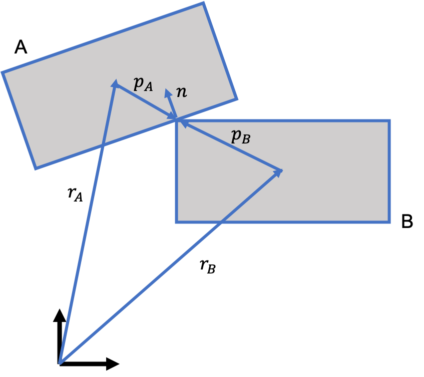
Collision detection is based on holding the constraint that the magnets cannot move in the direction where they would intersect more. Mathematically, we can arrive at this constraint:
$$ C = [(r_A+p_A)-(r_B+p_B)] $$ $$ C \cdot n > 0 \, (no \, penetration) $$ $$ C \cdot n < 0 \, (penetration) $$ $$ C \cdot n = 0 \, (blocks \, touching) $$We define \(n\) to be the unit normal pointing from block B to A. In the case where we have penetration, the vector \(C\) would be pointing in the opposite direction of \(n\). In the last equation, \(C=0\) and that's how we get the dot product to be 0.
We can then take the derivative of the dot product, and we obtain:
$$ \frac{d}{dt}(C\cdot n) = \frac{dC}{dt} \cdot n + C \cdot \frac{dn}{dt} \approx \frac{dC}{dt} \cdot n = 0 $$We can assume that \(n\) doesn't change and that we are interested in ensuring that the \(C\) vector doesn't move and result in more penetration so having \(\frac{dC}{dt} \cdot n = 0\) means that the block can move perpendicular to \(n\) but that's it. We then have:
$$ \frac{dC}{dt} \cdot n = [(v_A + \omega_A \times p_A) - (v_B + \omega_B \times p_B )] \cdot n $$ $$ = v_A \cdot n + \omega_A \cdot (p_A \times n) - v_B \cdot n - \omega_B \cdot (p_B \times n) $$ $$ = [n , p_A \times n , -n , - p_B \times n] \cdot [v_A , \omega_A , v_B , \omega_B] $$ $$ = J \cdot u = 0 $$We also don't want the collision or response to involve work. When something falls on a table and bounces, we don't say that the table did work on the object. We then have:
$$ P = F_c \cdot u = 0 $$ $$ F_c = [F_A , T_A , F_B , T_B] $$We then get:
$$ J \cdot u = 0 $$ $$ F_c \cdot u = 0 $$From our force and torque balance, we can write:
$$ m_A \frac{dv_A}{dt} = F_c(1) + F_{A,ext} $$ $$ I_A \frac{d\omega_A}{dt} = F_c(2) + T_{A,ext} $$ $$ m_B \frac{dv_B}{dt} = F_c(3) + F_{B,ext} $$ $$ I_B \frac{d\omega_B}{dt} = F_c(4) + T_{B,ext} $$Subscript \(ext\) refers to external forces and torques. We can integrate to get:
$$ m_A dv_A = \int (F_c(1) + F_A) dt $$ $$ I_A d\omega_A = \int (F_c(2) + T_A) dt $$ $$ m_B dv_B = \int (F_c(3) + F_B) dt $$ $$ I_B d\omega_B = \int (F_c(4) + T_B) dt $$Assuming a very short time duration for the impulse, the integral of \(F_A,T_A,F_B,T_B\) can be ignored. We then get:
$$ M \Delta u = F_C^T \Delta t = \lambda J^T $$The second equality comes from \(F_C \cdot u = 0\) and \(J \cdot u = 0\). We then have:
$$ F_c \cdot u = 0 $$ $$ J \cdot u = 0 $$ $$ M \Delta u = \lambda J^T $$We can say that \(F_c\) and \(J\) are \(1 \times n\) row vectors \(u\) is a \(n \times 1\) column vector. Then we can find:
$$ Mu = Mu_o + \lambda J^T $$ $$ u = u_o + \lambda M^{-1}J^T $$ $$ J u = 0 = J u_o + \lambda JM^{-1}J^T $$ $$ \lambda = - \frac{Ju_o}{JM^{-1}J^T} $$We see that \(\lambda\) is a scalar since \(Ju_o\) is a scalar (\(1 \times n * n \times 1\)) and the denominator, \(JM^{-1}J^T\), is (\(1 \times n * n \times n * n \times 1\)) which is also a scalar. We then find the response using:
$$ u = u_o + \lambda M^{-1}J^T $$So to implement the impulse response, it's actually pretty straightforward. The challenging part is finding \(J = [n , p_A \times n , -n , - p_B \times n]\), specifically \(p_A\) and \(p_B\). I wanted to keep things simple for this model but in reality, there will be multiple contact points most of the time so you would want something like:
$$ u = u_o + \frac{1}{N} \sum \lambda_i M^{-1}J_i^T $$where we sum over \(N\) contact points. It would be somewhat straightforward to expand to this from where I am but the model gets a little more complex. My results seemed fairly good so I'm just going to leave things where they are.
I'll give a description of how I found \(J\) since this might have been the part of the project I spent the most time. Finding \(n\) is easy compared to finding \(p_A\) and \(p_B\). I was originally thinking of when detecting a collision, to use a bisection search to find what the last direction is that doesn't result in a collision and then saying this is my direction. I ended up not doing that. Instead I use the distances (remember the projection of the blocks and the project of the center-to-center vector) along with a check on the dot product of that direction with the velocity vector. I end up selecting the direction that meets my distance criteria (the absolute value of the block projection minus the center-to-center projection must be less than some threshold) and the direction that maximizes the absolute value of the dot product of the direction and velocity vectors.
Finding \(p_A\) and \(p_B\) are more involved. The first thing to do is determine what the collision type is. I broke it down into four different types:
- Face-Face Collision: The two faces of the magnets are colliding
- Face-Edge with A Face: The face of Magnet A collides with the edge of Magnet B
- Face-Edge with B Face: The face of Magnet B collides with the edge of Magnet A
- Edge-Edge: Two edges of the magnets are colliding
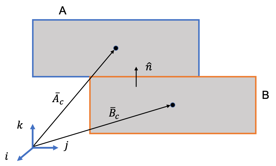
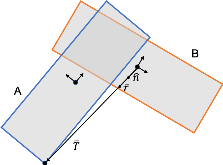
Physically, we only expect the overlapping type of collision since if the faces don't overlap, there won't be a collision. In the overlapping case, we look for the center of the overlap area and use that in our \(p_A\) and \(p_B\) calculations. We loop over the whole area of the block A face involved in the collision and use the overlapping points in our center of area equation:
$$ x_{cm} = \frac{1}{N} \sum^N_i x_i \, (for \, (x_i,y_i) \in A_{overlap} )$$ $$ y_{cm} = \frac{1}{N} \sum^N_i y_i \, (for \, (x_i,y_i) \in A_{overlap} )$$where \(N\) is the total number of overlap points. If a point is not in the overlap region, we don't include it. The above schematic illustrates how we determine if a point is within the overlap area. We first have the vector (\(T\)) from the center of Block B to the point we are testing. Then in that same direction (\(n\)) we find the vector the edge of block B in that direction (\(r\)). If the magnitude of \(r\) is greater than the magnitude of \(T\), we say that the point of interest is in the overlap area.
For the non-overlapping case, we know that \(p_A\) and \(p_B\) will point to the edges of each respective block. We find the center to center vector, (\T\), and need to be careful about the direction. We define the direction of \(T\) to point from Block B to Block A. We need to be careful about the direction because we want to search for the minimum distance and need to look on the proper edges. Defining the direction of \(T\) helps us do that.
Once we find the right edges to search on, we begin at the corner of the collision face of block A. We will have two edges that we are interested in and starting at the corner helps us find the right edge to search in (also the corner might be the point that results in the minimum distance).
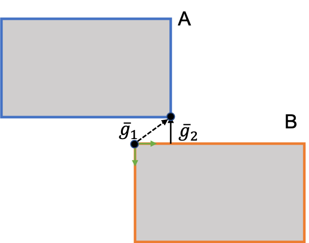
We then start at the corner of the collision face of block B and find the vector from the point on block A to the point on block B. We call this vector, the vector \(g\). We then find the magnitude of \(g\), called \(|g|\). We then move along one edge, calculate the magnitude of \(g\) there and also move along the other edge and calculate the magnitude of \(g\) there too. We find the derivative and move in the direction that minimizes the magnitude of \(|g|\). In this way, we find the point on B that minimizes the distance between the point on block A and the point on block B. After this, we essentially do the same thing on block A by finding the derivative of \(g\) and moving in that direction until we find the minimum \(g\) and the resulting points on block A and B lead to \(p_A\) and \(p_B\).
This is illustrated in the schematic below where we first start at the corner of block A and then initially find \(g\) (labeled \(g_1\) in the schematic) using the corner of block B. The derivative here says to move along the horizontal edge and we move in that direction until finding the minimum \(g\) (labeled \(g_2\) in the schematic). We would then find the derivative for the point on A but in this case, moving in either direction doesn't result in us minimizing \(g\) anymore so the calculation stops. Since the blocks are rectangular, we expect this to be a nice linear problem for every orientation.
The Face-Edge collision has two options: edge of A collides with face of B and edge of B collides with face of A. For both of these cases, we take the same approach. We first find the correct edge and face. We use a similar strategy to the non-overlapping face-face collision where we use the center to center vector \(T\), and specify it's direction from B to A. We then check the dot product with the block axes to determine what directions we are interested in and use this to pick the correct edge and face.
We then use a bisection search on the edge. We use the two end points as our initial min and max. For each point on the edge, we search along the face using the derivative of (\g\) until we minimize \(g\). We then step slightly in each direction on the edge to find the deritative of \(g\) from the edge point of view. We use this derivative to update our bounds on the bisection search. The process is illustrated below
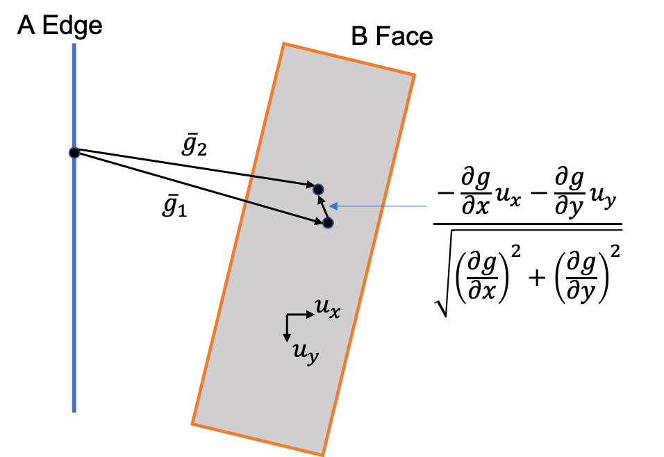
Assume we have a point on edge A we are starting with. We find the point on the face that minimizes \(g\) which is the vector from the point on the edge of A to a point on the face of B. We then find the derivative in each direction and move in the direction that decreases \(g\) (in the schematic this is shown by going from \(g_1\) to \(g_2\)). In the next step, we would step along the edge of A in both directions to find that derivative and then use that derivative to adjust our bounds in the bisection search.
The Edge-Edge case is actually the easiest and compared to the others, will only have one contact point (unless the edges are parallel and colliding which would be a very unusual, and not expected case). With the Edge-Edge case, we have an analytical solution to the contact points.
To get the solution for \(p_A\) and \(p_B\), we start with the figure below:
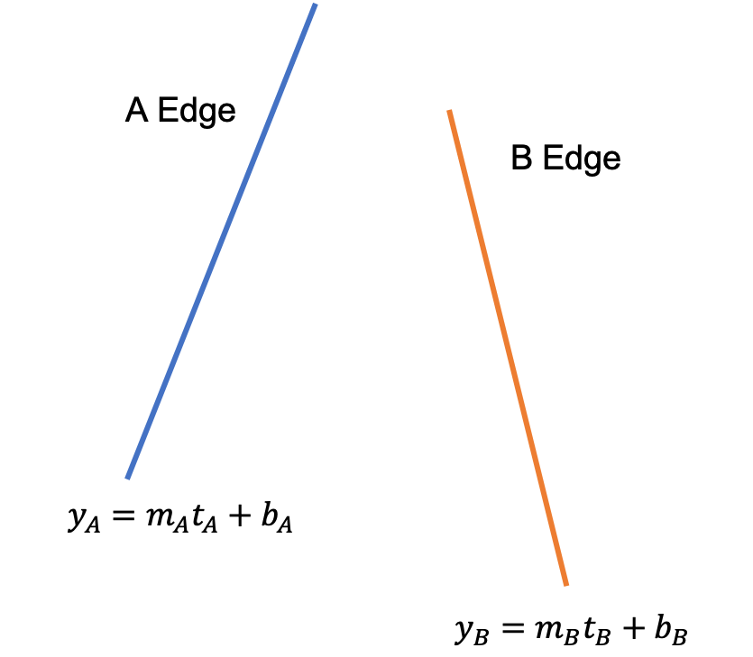
We have two equations, one for each edge:
$$ y_A = m_A t_A + b_A $$ $$ y_B = m_B t_B + b_B $$Here, \(y\), \(m\), and \(b\) are 3x1 column vectors and \(t\) is a scalar. We can then say that the vector between one point on edge A and one point on edge B is:
$$ F = (y_A - y_B) $$The magnitude is then:
$$ |F|^2 = g = (y_A - y_B)^2 $$To find the minimum distance, we want to find:
$$ \frac{\partial g}{\partial t_A} = 0 $$ $$ \frac{\partial g}{\partial t_B} = 0 $$We get:
$$ \frac{\partial g}{\partial t_A} = 2 (m_A^2t_A - m_Am_Bt_B + m_Ab_A - m_Ab_B) = 0 $$ $$ \frac{\partial g}{\partial t_B} = 2 (m_B^2t_B - m_Am_Bt_A + m_Bb_B - m_Bb_A) = 0 $$We then have two equations and two unknowns. We can solve this linear equation of systems:
$$ \begin{bmatrix} m_A^2 & -m_Am_B \\ -m_Am_B & m_B^2 \end{bmatrix} \begin{bmatrix} t_A \\ t_B \end{bmatrix} = \begin{bmatrix} -m_A (b_A-b_B) \\ m_B (b_A - b_B) \end{bmatrix} $$ $$ \begin{bmatrix} t_A \\ t_B \end{bmatrix} = \begin{bmatrix} m_A^2 & -m_Am_B \\ -m_Am_B & m_B^2 \end{bmatrix} ^{-1} \begin{bmatrix} -m_A (b_A-b_B) \\ m_B (b_A - b_B) \end{bmatrix} $$We include limits to make sure that \(t\) doesn't exceed the edge beginning or end. This section summarizes how we find \(p_A\) and \(p_B\).
Model Details and Example
This section describes the model details and how the model was put together. The schematic below gives an overview of how the model works.
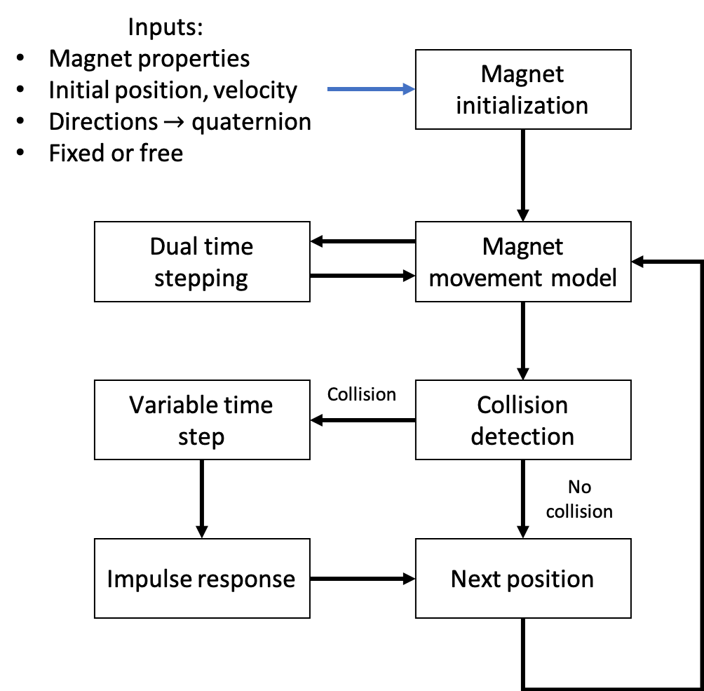
The user needs to first specify the magnet properties and initial conditions. The model then takes these properties and creates a magnet object with those properties. You can also fix one magnet (so it's sort of like you are holding one magnet still and letting the other model respond).
After this, we solve the equations of motion utilizing dual time stepping (again). When a collision is detected, we use a bisection search to find the time when our models initially collide. The model will output the time when a collision occurs and will also output the type of collision (Face-Face, etc.). We then calculate our impulse response and we move into the next iteration of the model.
The model will then generate a video of the simulation and show the initial position and end position of the simulation. If a collision is detected, the model is most likely a variable time stepping solution since we change the time step during a collision. The video function only wants a constant time step so we first need to alter our model time step to a constant time step time vector.
We also need to be careful about our frame rate (fps = frames per second). My computer is only capable of such a frame rate speed and since the magnet responses are very quick, we can only watch the videos at like 1 % speed. If we try to watch full speed, the computer can't keep up and the computer shows at some reduced fps. This was messing me up for a little. The interactive video utilizes the interval instead of a frame rate. The interval is the number of ms between frames so we get this with interval = 1000 / fps.
I'm going to show the same example above first. I was playing around with the model trying to find an orientation where the magnets would snap together rather than repel each other. The initial positions are shown below:
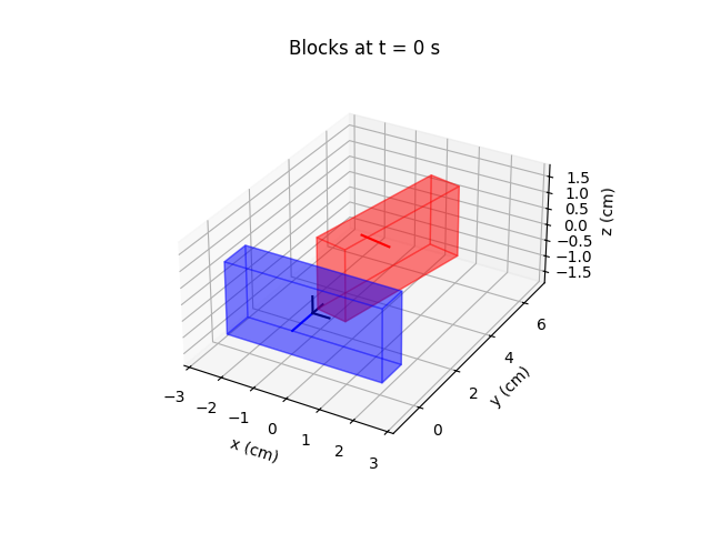
We hold the blue magnet still and I was playing with the red magnet (particularly the angle it makes with the blue magnet) until I got the magnets to snap together. The final positions are shown below:
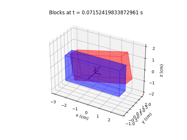
I believe in a perfect simulation, the magnets would still be aligned instead of the red magnet being at a little angle. I think this is due the impulse response using one \(p_A\) and one \(p_B\). If I took a weighted approach, I think the magnets would be more aligned. Maybe one day I will expand and test that.
Notice the final time is 0.07 s or 70 ms which is very fast. This aligns with our experience with block magnets and how fast they can move. A video at 1 % speed is below:
I think the model is actually pretty cool and seems to capture the physics a lot better than I maybe thought it would be, potentially validating some of my thoughts earlier in this project. This is probably the most advanced side project model I have built. I have built some involved physics models for work that are close to the level of work that was needed for this. I did cut some corners to speed up the project and clearly spent very little time validating or fine tuning everything. I am happy with how this turned out though.
I know the math worked out but it's still cool to see the face-edge collision and the response. It's cool to actually see the red magnet bounce off the blue. I'm not sure if that actually happens or not (and I kinda doubt my phone camera can capture that. There other things I could try like putting some chalk on the red magnet edge and seeing if it leaves a mark on the blue magnet where the model suggests).
I still have some work to do here and would like to look at other examples to see if I can find any errors or break the model. I am knee deep in an international move so some of that might have to wait til later ...
Model vs Experiment
Coming soon!