Miscellaneous
Random projects, experiments, and notes that don’t fit neatly into modeling:
Electric Field from Moving Charge
(Feynman Volume II Derivation)
On page 21-1 in Volume II of The Feynman Lectures on Physics, the equation for the electric field of an electron moving in an arbitrary direction (shown on right) is presented and some of the details about the equation are discussed.
Further along (page 21-11) Feynman sort of challenges the reader in the footnote to fully derive the equation and I thought it would be useful to try to derive the equation and that it would be good practice
Complete derivation with all details: Electric Field from Moving Charge Derivation
Rope hanging from helicopter at constant speed
I came across this video on youtube by Veritasium that shows a phsyics problem where a helicopter is moving at constant speed and asks if a rope is dangling from the helicopter, what shape is the rope making?
The prompt makes it clear to not neglect air friction (drag). See the problem below. The question gives different options for the shape of the rope.

I think most people would select (B) or (C). Maybe you would pick (A) and say you assume a very heavy rope and a very low speed for the helicopter.
I thought it could be a cool exercise to see how I could find my answer analytically (if possible). To do this, I looked at a small (infitesimal) segment of robe and the force balance on that segment (free body diagram). This is shown below (note I draw the rope as a straight line but I could have drawn this with any arbitary shape - it's not important in the derivation).

In the above schematic, \(T\) is tension, \(F_g\) is the force of gravity, and \(F_D\) is the drag force (air friction).
We assume the rope has length \(L\), the rope has uniform mass density \(\lambda\) (mass per unit length), and that the rope segment angle \(\theta\) can vary as a function of position on the rope.
We can first find the forces in the x direction (we assume the helicopter is moving in the negative \(x\) direction with speed \(u\)). We get:
$$ \sum F_x = -T_{x,y}cos(\theta) + T_{x+dx,y+dy}cos(\theta) + F_D $$Expanding \(T_{x+dx,y+dy}\) using Taylor series gives:
$$ \sum F_x = -T_{x,y}cos(\theta) + T_{x,y}cos(\theta) + \frac{\partial T_{x,y}}{\partial x} cos(\theta) dx + \frac{\partial T_{x,y}}{\partial y} cos(\theta) dy + F_D $$ $$ \sum F_x = \frac{\partial T}{\partial x} cos(\theta) dx + \frac{\partial T}{\partial y} cos(\theta) dy + \frac{1}{2} C_D \rho_{air} u^2 dy $$We simplify the drag term by assuming that \(\frac{1}{2} C_D \rho_{air} u^2\) is the same for all rope segments. We also assume that we are at steady state so our force summation equals 0.
$$ \frac{\partial T}{\partial x} cos(\theta) dx + \frac{\partial T}{\partial y} cos(\theta) dy + K_D dy = 0 $$We do the same thing in the \(y\) direction and obtain:
$$ \sum F_y = -T_{x,y} sin(\theta) + T_{x+dx,y+dy} sin(\theta) + F_g $$Expanding and simplifying, dropping subscripts for tension, substituting in for gravity, and equating to 0 gives:
$$ \frac{\partial T}{\partial x} sin(\theta) dx + \frac{\partial T}{\partial y} sin(\theta) dy + \lambda g ds = 0 $$Note that for gravity, we have \(ds\) since gravity acts on the whole segment. We now have our two equations:
$$ \frac{\partial T}{\partial x} cos(\theta) dx + \frac{\partial T}{\partial y} cos(\theta) dy + K_D dy = 0 $$ $$ \frac{\partial T}{\partial x} sin(\theta) dx + \frac{\partial T}{\partial y} sin(\theta) dy + \lambda g ds = 0 $$From the geometry, we have \(\frac{dy}{dx} = tan(\theta)\) and that \(ds=\frac{dx}{cos(\theta)}=\frac{dy}{sin(\theta)}\). We can divide both equations by \(dx\) and substitute in for \(ds\) to get:
$$ \frac{\partial T}{\partial x} cos(\theta) + \frac{\partial T}{\partial y} cos(\theta) \frac{dy}{dx} + K_D \frac{dy}{dx} = 0 $$ $$ \frac{\partial T}{\partial x} sin(\theta) + \frac{\partial T}{\partial y} sin(\theta) \frac{dy}{dx} + \lambda g \frac{1}{cos(\theta)} = 0 $$We then use \(\frac{dy}{dx}=tan(\theta)\) to get:
$$ \frac{\partial T}{\partial x} cos(\theta) + \frac{\partial T}{\partial y} cos(\theta) tan(\theta) + K_D tan(\theta) = 0 $$ $$ \frac{\partial T}{\partial x} sin(\theta) + \frac{\partial T}{\partial y} sin(\theta) tan(\theta) + \lambda g \frac{1}{cos(\theta)} = 0 $$Solving the second equation for \(\frac{\partial T}{\partial y}\), we find:
$$ \frac{\partial T}{\partial y} = -\frac{\partial T}{\partial x} \frac{1}{tan(\theta)} - g \lambda \frac{1}{sin^2(\theta)} $$Plugging this into the first equation gives:
$$ \frac{\partial T}{\partial x} cos(\theta) + ( -\frac{\partial T}{\partial x} \frac{1}{tan(\theta)} - g \lambda \frac{1}{sin^2(\theta)}) cos(\theta) tan(\theta) + K_D tan(\theta) = 0 $$Expanding gives:
$$ \frac{\partial T}{\partial x} cos(\theta) -\frac{\partial T}{\partial x} cos(\theta) - g \lambda \frac{1}{sin(\theta)} + K_D tan(\theta) = 0 $$We then get:
$$ g \lambda = K_D tan(\theta) sin(\theta) = K_D \frac{sin^2(\theta)}{cos(\theta)} = K_D \frac{1 - cos^2(\theta)}{cos(\theta)}$$We then can divide both sides by \(K_D\) and say \(\alpha = \frac{g \lambda}{K_D}\) and obtain:
$$ cos^2(\theta) + \alpha \, cos(\theta) - 1 = 0 $$We have a quadratic equation now and can solve for \(cos(\theta)\):
$$ cos(\theta) = \frac{-\alpha \pm \sqrt{\alpha^2 - 4}}{2} $$We have found a solution for the angle that only depends on gravity, rope mass density, and drag. All of these are assumed constant and gives us a constant angle so we conclude we have the straight line which is answer (B). This is also what the youtube video above shows from Veritasium.
There is more we can do based on our findings. Below is a table for values of \(\alpha\) and \(\frac{-\alpha \pm \sqrt{\alpha^2 - 4}}{2}\). From \(\alpha\), we know that \(\alpha=0\) (or the limit as \(\alpha\) approaches 0) would correspond to a very, very light rope or a rope situation with very high drag. We know. that \(\alpha=\infty\) (or the limit as \(\alpha\) approaches \(\infty\)) would correspond to a scenario with a very low drag coefficient or a very, very heavy rope. Lets look at the results and what physics the results suggest
| \(\alpha\) | \(\frac{-\alpha + \sqrt{\alpha^2 - 4}}{2}\) | \(\frac{-\alpha - \sqrt{\alpha^2 - 4}}{2}\) |
|---|---|---|
| 0 | 1 | 0 |
| \(\infty\) | 0 | -\(\infty\) |
From the table, we see that that \(\frac{-\alpha + \sqrt{\alpha^2 - 4}}{2}\) corresponds to our physical solution and while \(\frac{-\alpha - \sqrt{\alpha^2 - 4}}{2}\) is also a mathematical solution to the quadratic, it's not an actual physical solution since \(cos(\theta)\) is never \(-\infty\). Now we can check what values of \(\alpha\) correspond to what values of \(\theta\) and check our physical reasoning. We said above that when \(\alpha\) approaches 0, it represents a very light rope so we would expect \(\theta\) to also approach 0 meaning the rope is so light that any air resistance pushes the rope to be horizontal and be parallel with the ground. When \(\alpha\) approaches \(\infty\) we expect a very heavy rope with small air resistance so that the rope falls straight down giving us a \(\theta\) of 90 deg. In the table, below we calculate what values of \(\alpha\) give us what values of \(\theta\).
| \(\alpha\) | \(cos(\theta)=\frac{-\alpha + \sqrt{\alpha^2 - 4}}{2}\) | \(\theta (deg)\) |
|---|---|---|
| 0 | 1 | 0 |
| \(\infty\) | 0 | 90 |
We see that the \(\theta\) and \(\alpha\) values are consistent with our physical understanding.
The last thing we can look is checking the tension in the rope at different segments. We create a similar schematic to the one above (shown below):

We can again look at a small segment of the rope. We do the force balance in the \(s\) direction:
$$ \sum F_s = -T_s + T_{s+ds} + F_D cos(\theta) + F_g sin(\theta) $$ $$ \frac{dT}{ds} ds + K_D cos(\theta) dy + \lambda g sin(\theta) ds = 0 $$ $$ \frac{dT}{ds} ds + K_D cos(\theta) sin(\theta) ds + \lambda g sin(\theta) ds = 0 $$ $$ \frac{dT}{ds} + K_D cos(\theta) sin(\theta) + \lambda g sin(\theta) = 0 $$ $$ \frac{dT}{ds} = - K_D cos(\theta) sin(\theta) - \lambda g sin(\theta) = C_1 $$ $$ T_s = C_1 s + C_2 $$We now want to find \(C_2\). We know that the tension as we approach the end of the rope will be 0 since there will be no gravity or drag force, so no tension force:
$$ T(s=L) = C_1 L + C_2 = 0 $$ $$ C_2 = - C_1 L $$ $$ T_s = C_1 s - C_1 L = C_1 (s-L) $$ $$ T_s = -[K_D cos(\theta) sin(\theta) + \lambda g sin(\theta)] (s-L) $$ $$ T_s = [K_D cos(\theta) sin(\theta) + \lambda g sin(\theta)] (L-s) $$There's a couple points to make here. First, tension is acting in the direction we assumed on our force balance (we know that \(0 \le \theta \le 90 \; deg.\) so that all parameters in the [ ] are positive). Any segment of rope that has it's end as the end of the rope will have gravity and air friction pulling in the \(s\) direction with tension pulling in the \(-s\) direction. We basically have tension in the rope due to gravity and air friction. We also note that tension is proportional to distance along the length of rope.
It's cool that such a simple problem can be very interesting.
Train Coupling as Spring, Mass, Dampener
In an interview a while back I was asked how analyze the coupling between trains. I forget what the analysis was supposed to be getting at it but the question was more about how to model the situation so using a free body diagram to show the forces and then model the coupling as a spring and damper so you end up with two masses and a spring and damper between them in the simplest case. The interviewer described how they used Simscape to model this and my first impression was that might be a little overkill so I decided to look at how you could do a simple model (that might give some insight) without using Simscape.
I think the actual application that would require this type of analysis might be where you are connecting train cars and looking at what speed the trains should be at. I assume one set is stationary and the other car is moving towards the stationary set to connect. So we have a stationary car and then a moving car (something has to cause the moving car to move but I ignore this). The other application is how to accelerate a set of trains so we can look at that by applying a force to one of the trains. The scenario for two cars is shown below.
In the end I could see how Simscape could be useful depending on the situation as the model can get a little complicated if you start looking at many cars. I ended up comparing 5 methods for modeling the two car scenario, looked at the case where the coupling is constrained (how much can it extend and compress), looked at the conservation of energy, and then compared the max. force on the coupling and total energy dissipation through the damper as a function of initial speed. This problem became fairly involved and I could have moved it to the Modeling Section but since I never had a good objective for this, I keep it here.
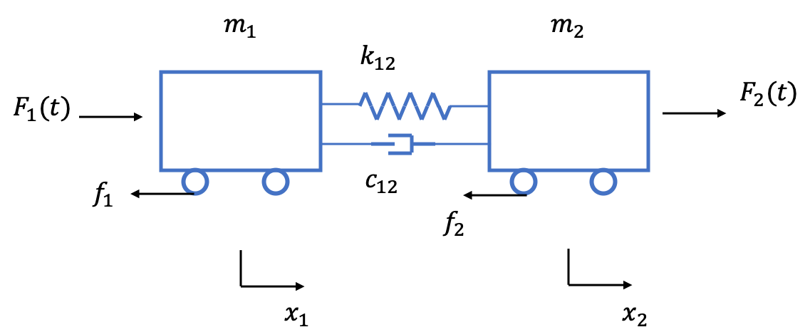
In the above, we have \(m_1\) and \(m_2\) as our train masses, and for each train we have an external force \(F\) and a constant friction coefficient \(f\). Connecting both trains is our spring, \(k_{12}\), and our damper, \(c_{12}\). Note the positive \(x_1\) and \(x_2\) directions are both in the right direction in the schematic.
The force balance for train car 1 is shown below.
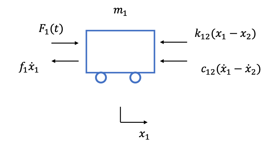
The force balance for train 2 is very similar except the force from the spring and damper are acting in the other direction. We then have:
$$ m_1 \frac{d \dot{x}_1}{dt} = -k_{12}(x_1-x_2) - c_{12}(\dot{x}_1-\dot{x}_2) - f_1 \dot{x}_1 + F_1(t) $$ $$ m_2 \frac{d \dot{x}_2}{dt} = k_{12}(x_1-x_2) + c_{12}(\dot{x}_1-\dot{x}_2) - f_2 \dot{x}_2 + F_2(t) $$We can make the friction force proportional to the normal force using \(f=\mu m g\). We multiply by the velocity so that we have no friction force when the car isn't moving.
We see that we can put this in state space form:
$$ \dot{x} = Ax + Bu $$For us we have (I don't use bars to denote vectors but it should be implied in this problem that \(x\) and \(u\) are generally vectors and \(A\) and \(B\) are generally matrices):
$$ x = \begin{bmatrix} x_1 \\ x_2 \\ \dot{x}_1 \\ \dot{x}_2 \end{bmatrix} \; , \; A = \begin{bmatrix} 0 & 0 & 1 & 0 \\ 0 & 0 & 0 & 1 \\ -\frac{k_{12}}{m_1} & \frac{k_{12}}{m_1} & -\frac{f_1+c_{12}}{m_1} & \frac{c_{12}}{m_1} \\ \frac{k_{12}}{m_2} & -\frac{k_{12}}{m_2} & \frac{c_{12}}{m_2} & -\frac{f_2+c_{12}}{m_2} \end{bmatrix} \; , \; B = \begin{bmatrix} 0 & 0 \\ 0 & 0 \\ \frac{1}{m_1} & 0 \\ 0 & \frac{1}{m_2} \end{bmatrix} \; , \; u = \begin{bmatrix} F_1(t) \\ F_2(t) \end{bmatrix}$$We can solve this in many different ways that we explore below. We can also include limits on how \(x_1\) and \(x_2\) can change. We are modeling the coupling as a spring and damper so we can have \( l_{min} \le (x_2-x_1) \le l_{max} \) too. Using the state space model, we can solve this explicitly and also implicitly using dual time stepping. To explore other ways, we can find the discrete state space form. We won't look to solve this analytically since we will need to diagonalize the state matrix and it will get a little messy. To get the discrete state space form, we do the following:
$$ \dot{x} = Ax + Bu $$ $$ e^{-At} \dot{x} = e^{-At} Ax + e^{-At} Bu $$ $$ d(e^{-At}x) = e^{-At} Bu $$ $$ e^{-At}x - x_0 = \int_0^t e^{-A\tau} Bu d\tau $$ $$ x = e^{At} x_0 + \int_0^t e^{A(t-\tau)} Bu d\tau $$We can then define \(x[k]=x(kT)\) where \(T\) is our time increment. We also have \(x[k+1]=x((k+1)T)\). We then can say:
$$ x[k] = e^{AkT} x_0 + \int_0^{kT} e^{A(kT-\tau)} Bu d\tau $$and
$$ x[k+1] = e^{A(k+1)T} x_0 + \int_0^{(k+1)T} e^{A((k+1)T-\tau)} Bu d\tau $$ $$ = e^{AT} e^{AkT} x_0 + \int_0^{kT} e^{A((k+1)T-\tau)} Bu d\tau + \int_{kT}^{(k+1)T} e^{A((k+1)T-\tau)} Bu d\tau $$ $$ = e^{AT} e^{AkT} x_0 + e^{AT}\int_0^{kT} e^{A(kT-\tau)} Bu d\tau + \int_{kT}^{(k+1)T} e^{A((k+1)T-\tau)} Bu d\tau $$ $$ = e^{AT} ( e^{AkT} x_0 + e^{AT}\int_0^{kT} e^{A(kT-\tau)} Bu d\tau ) + \int_{kT}^{(k+1)T} e^{A((k+1)T-\tau)} Bu d\tau $$ $$ = e^{AT} x[k] + \int_{kT}^{(k+1)T} e^{A((k+1)T-\tau)} Bu d\tau $$Focusing on the last term on the RHS, we can make substitution \(v=(k+1)T-\tau\) and obtain:
$$ \int_{kT}^{(k+1)T} e^{A((k+1)T-\tau)} Bu d\tau = - \int_{T}^{0} e^{Av} Bu dv$$ $$ = \int_{0}^{T} e^{Av} Bu dv $$If we then assume that \(B\) is constant and \(u\) is constant over our \(T\) interval, we have:
$$ \int_{0}^{T} e^{Av} Bu dv = ( \int_{0}^{T} e^{Av} dv ) \, Bu[k]$$ $$ = A^{-1} (e^{AT} - I) Bu[k] $$So we then have:
$$ x[k+1] = e^{AT} x[k] + A^{-1} (e^{AT} - I) Bu[k] $$We then have 5 methods to explore:
- Explicit Method
- Dual Time Stepping
- Discrete with One Riemann Sum
- Discrete with SVD Inverse
- Discrete using Pade Approximation
Explicit Method
The explicit method is the easiest to implement. For this we just use:
$$ \dot{x}_k = \frac{1}{dt} (x_{k+1}-x_k) $$and we solve this explicitly at each time step using the values at the past time step. In general, this method can be less stable and lead to errors especially if the time step is large
Dual Time Stepping
This method is very cool and I would like to eventually implement it in my CFD Project. In this method, we use an additional psuedo-time step to solve the differential equation. This can be illustrated as:
$$ \dot{x} = Ax + Bu $$We then discretize and say:
$$ \frac{1}{\Delta t}(x_{k+1}-x_k) = Ax_{k+1} + Bu_{k+1} $$We then have an implicit equation, and we can bring both terms to the same side so we have:
$$ \frac{1}{\Delta t}(x_{k+1}-x_k) - ( Ax_{k+1} + Bu_{k+1} ) = 0 $$Introducing dual time stepping, we obtain:
$$ \frac{dx_{k+1}}{dt'} - \frac{1}{\Delta t}(x_{k+1}-x_k) - ( Ax_{k+1}^{n} + Bu_{k+1} ) = 0 $$As \(t'\) approaches \(\infty \), we converge on the solution so we can use explict pseudo-time stepping:
$$ \frac{1}{\Delta t'} (x_{k+1}^{n+1} - x_{k+1}^{n}) - \frac{1}{\Delta t}(x_{k+1}^{n}-x_k) - ( Ax_{k+1}^{n} + Bu_{k+1} ) = 0 $$We also introduce some limitations on the psuedo-time step, \(\Delta t'\), so that we don't have oscillations. So dual time stepping is an implict method and we can tolerate larger time steps comapred to the explicit method and should in general have a more stable and robust solver.
Discrete with One Riemann Sum
In this method, we start with:
$$ x[k+1] = e^{AT} x_0 + (\int_{0}^{T} e^{Av} dv) \, Bu[k]$$If we assume that our time step, \(T\), is small enough, we can appoximate \(\int_{0}^{T} e^{Av} dv\) as \(T \), \(e^{AT}T\), or \(e^{\alpha T}T\) where \(\alpha \le 1\). We expect this method to be similar to the explicit method. This method will be sensitive to the time step and can be, in general, not stable.
Discrete with SVD Inverse
In this method, we use:
$$ x[k+1] = e^{AT} x[k] + A^{-1} (e^{AT} - I) Bu[k] $$However, due to the symmetry in our model, we can see how \(A\) can be singular. To alleviate this, we can use the SVD of A and find the inverse using the SVD. The SVD decomposition of a matrix is defined as:
$$ A = U \Sigma V^H $$The SVD can be very useful. \(U\) and \(V\) are both unitary matrices (meaning \(UU^H=I\)) and \(\Sigma\) is a matrix with the singular values of \(A\) along the diagonal in descending order. The SVD has the advantage of working for non-square matrices and you can find the pseudo-inverse for singular matrices. One of these days, I will look into more detail about the SVD, particularly in how to find the singular values. There's a lot we could say here, but we find the SVD using Numpy in python then we can use the transpose (or conjugate transpose in general) of \(U\) and \(V\) and take the recripocal of the singular values in \(\Sigma\).
$$ A^+ = V \Sigma^+ U^H $$Here, \(A^+\) is the psuedo-inverse and \(\Sigma^+\) has the recripocal of the singular values of \(A\) along its diagonal.
Discrete with Pade Approximation
In this method, we again use:
$$ x[k+1] = e^{AT} x[k] + A^{-1} (e^{AT} - I) Bu[k] $$This time, we can expand \(e^{AT} = \sum_{k=0}^{\infty} \frac{(AT)^{k}}{k!}\). When we plug this in, we get:
$$ x[k+1] = e^{AT} x[k] + A^{-1} (\sum_{k=0}^{\infty} \frac{(AT)^{k}}{k!} - I) Bu[k] $$ $$ = A^{-1} (I + \sum_{k=1}^{\infty} \frac{(AT)^{k}}{k!} - I) Bu[k] $$ $$ = \sum_{k=1}^{\infty} \frac{A^{k-1}T^{k}}{k!} Bu[k] = \sum_{k=0}^{\infty} \frac{A^{k}T^{k+1}}{(k+1)!} $$We then can use a Pade approximation for \( \sum_{k=0}^{\infty} \frac{A^{k}T^{k+1}}{(k+1)!} \). This will be good practice for understanding the Pade approximation. We will find a [2/2] Pade approximation. What we will have is:
$$ m_0 + m_1 A + m_2 A^2 + m_3 A^3 = \frac{a_0 + a_1 A + a_2 A^2}{1 + b_1 A + b_2 A^2} $$The first thing we want to do is expand the denominator the Pade approximation to get a geometric series:
$$ \frac{1}{1 + b_1 A + b_2 A^2} = c_0 + c_1 A + c_2 A^2 + c_3 A^3 + ... $$ $$ 1 = (1 + b_1 A + b_2 A^2)(c_0 + c_1 A + c_2 A^2 + c_3 A^3 + ...) $$ $$ 1 = c_0 + (c_1 + b_1c_0)A + (c_2 + b_1c_1 + b_2c_0)A^2 + (c_3 b_1c_2 b_2c_1)A^3 + (c_4 + b_1c_3 + b_2c_2)A^4 + ... $$We then have:
$$ c_0 = 1 $$ $$ c_1 = -b_1 $$ $$ c_2 = -b_s1c_1 - b_2c_0 = b_1^2 - b_2 $$ $$ c_3 = -b_1c_2 - b_2c_1 = -b_1(b_1^2 - b_2) - b_2(-b_1) = -b_1^3 + 2b_1b_2 $$ $$ c_4 = -b_1c_3 - b_2c_2 = -b_1(-b_1^3 + 2b_1b_2) - b_2(b_1^2 - b_2) $$ $$ c_4 = b_1^4 - 2b_1^2b_2 - b_1^2b_2 + b_2^2 = b_1^4 - 3b_1^2b_2 + b_2^2 $$Going back to our pade approximation, we have:
$$ m_0 + m_1 A + m_2 A^2 + m_3 A^3 = \frac{a_0 + a_1 A + a_2 A^2}{1 + b_1 A + b_2 A^2} $$ $$ = (a_0 + a_1 A + a_2 A^2) (c_0 + c_1 A + c_2 A^2 + c_3 A^3 + ...) $$ $$ = a_0c_0 + (a_0c_1 + a_1c_0) A + (a_0c_2 + a_1c_1 + a_2c_0) A^2 + (a_0c_3 + a_1c_2 + a_2c_1) A^3 $$ $$ + (a_0c_4 + a_1c_3 + a_2c_2) A ^ 4 + ... $$I knew this already, but we can check here that we have 5 unknowns \(a_0,a_1,a_2,b_1,b_2\) and we have 5 equations. We can substitute in for our \(c_i\) values:
$$ m_0 + m_1 A + m_2 A^2 + m_3 A^3 = a_0 + (-a_0b_1 + a_1) A + [a_0(b_1^2-b_2) - a_1b_1 + a_2] A^2$$ $$ + [a_0(-b_1^3 + 2b_1b_2) + a_1(b_1^2 - b_2) - a_2b_1] A^3 $$ $$ + [a_0(b_1^4 - 3b_1^2b_2 + b_2^2) + a_1(-b_1^3 + 2b_1b_2) + a_2(b_1^2 - b_2)] A ^ 4 + ... $$We now say:
$$ a_0 = m_0 $$ $$ -a_0b_1 + a_1 = m_1 $$ $$ a_0(b_1^2-b_2) - a_1b_1 + a_2 = m_2 $$ $$ a_0(-b_1^3+2b_1b_2) + a_1(b_1^2-b_2) - a_2b_1 = m_3 $$ $$ a_0(b_1^4 - 3b_1^2b_2 + b_2^2) + a_1(-b_1^3 + 2b_1b_2) + a_2(b_1^2 - b_2) = m_4 $$This can be solved in a couple different ways. We can say that we have \(\bar{v}=(a_0,a_1,a_2,b_1,b_2)^T\) and that we have \(F(\bar{v})=\bar{g}=(m_0,m_1,m_2,m_3,m_4)^T\). We then can say:
$$ F(\bar{v}) ~= F(\bar{v}_{n}) + \frac{dF}{d\bar{v}}(\bar{v}_{n+1}-\bar{v}_{n}) = \bar{g} $$We solve this for \(\bar{v}_{n+1}\):
$$ \bar{v}_{n+1} =\bar{v}_{n} + (\frac{dF}{d\bar{v}})^{-1} ( \bar{g} - F(\bar{v}_{n}) ) $$For \(\frac{dF}{d\bar{v}}\), we have:
$$ \frac{dF}{d\bar{v}} = \begin{bmatrix} 1 & 0 & 0 & 0 & 0 \\ -b_1 & 1 & 0 & -a_0 & 0 \\ b_1^2-b_2 & -b_1 & 1 & 2a_0b_1 - a_1 & -a_0 \\ -b_1^3+2b_1b_2 & b_1^2-b_2 & -b_1 & \begin{aligned} -3a_0b_1^2 + 2a_0b_2 \\ + \; 2a_1b_1 - a_2 \end{aligned} & 2a_0b_1 - a_1 \\ b_1^4 - 3b_1^2b_2 + b_2^2 & -b_1^3 + 2b_1b_2 & b_1^2 - b_2 & \begin{aligned} 4a_0b_1^3-6a_0b_1b_2- 3a_1b_1^2 \\ + \; 2a_1b_2 + 2a_2b_1 \end{aligned} & \begin{aligned} -3a_0b_1^2 + 2a_0b_2 \\ + \; 2a_1b_1 - a_2 \end{aligned} \end{bmatrix} $$We iterate to find the parameters, and then we ultimately have:
$$ x[k+1] = e^{AT} x[k] + \sum_{k=0}^{\infty} \frac{A^{k}T^{k+1}}{(k+1)!} Bu[k] $$where \(\sum_{k=0}^{\infty} \frac{A^{k}T^{k+1}}{(k+1)!} \) is approximated using the [2/2] Pade approximation we found above.
Method Comparison
The plot below shows the state vector comparison between the five methods for the scenario where mass 2 has an initial velocity moving to the left and there is a sinusoidal force on the first mass. I also include \(x_2-x_1\) which is the coupling length essentially or the distance between the cars. Below, I look at constraining this geometry assuming the trains connect and then the cars can only be so close and so far away from each other corresponding to how much the coupling can expand and compress.
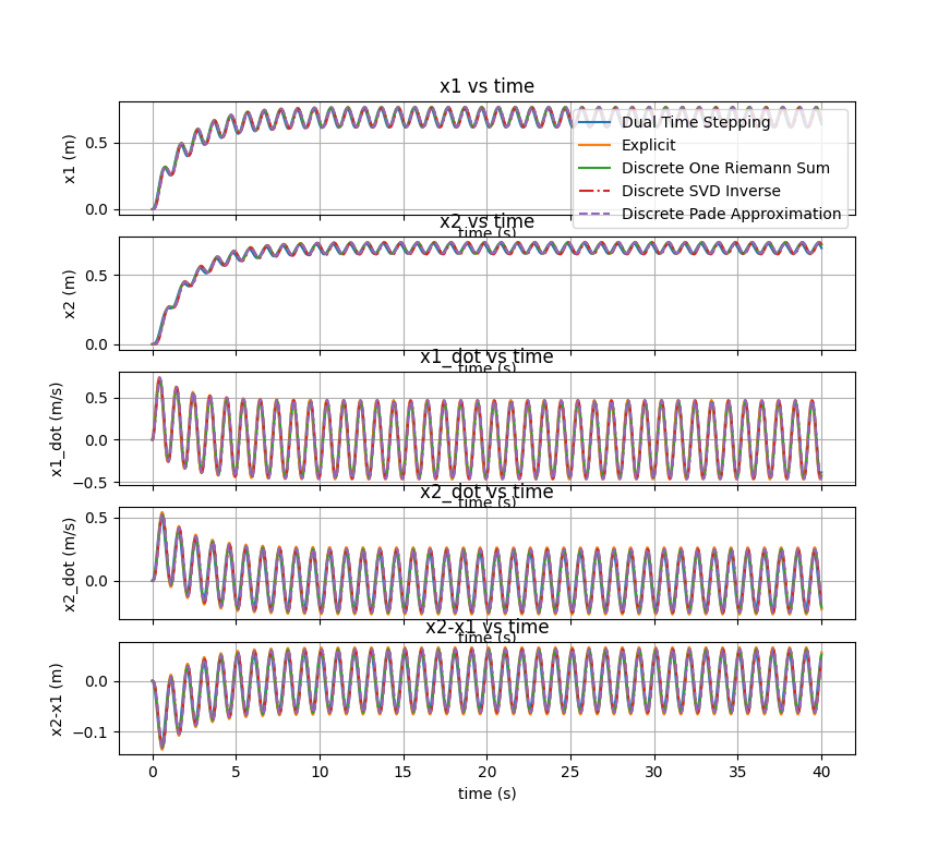
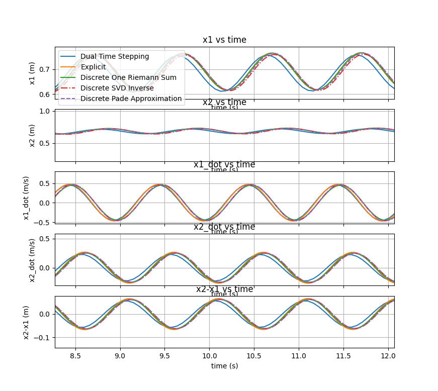
We see that all the methods produce about the same results which isn't too surprising since the model is not very complicated. It was cool to get almost the same result using several different methods. The plot on the left is the whole simulation (40 seconds) and the one on the right zooms in on a shorter time segment to better appreciate the differences between the methods.
Below is a plot showing the force on the coupling from the spring, distance between cars, coupling, and relative speed of the cars (to each other).
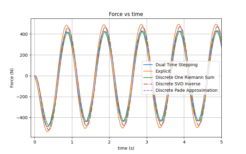
The methods again produce very similar results with the Explicit method giving the highest amplitude and Dual Time Stepping giving the smallest. This isn't too surprising since the Explicit method is a little more unstable than the Dual Time Stepping method.
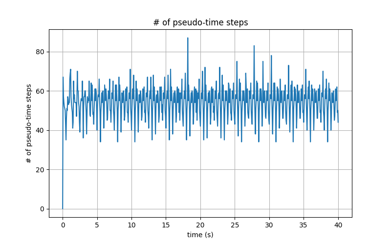
Below, I show the number of pseudo-time steps at each time step for the Dual Time Stepping method. It's interesting to see how many times the Dual Time Stepping method iterates per time step, especially compared to the Explicit method which only interates once.
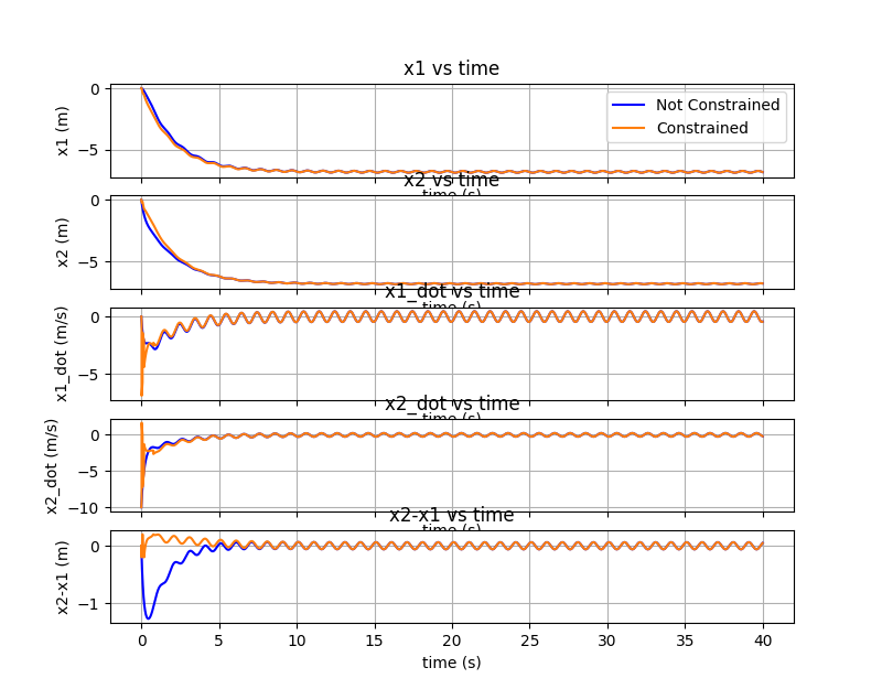
Constrained Geometry
I wanted to look at the scenario where the coupling geometry is constrained meaning it can only expand and compress so much. I would then have:
$$ l_{min} \le (x_2-x_1) \le l_{max} $$To do this, I assume that the collisions are perfectly elastic so I conserve both momentum and energy. I also iterate on my time step when I exceed my bounds. I use a bisection search method to find the time step that results in my distance between the cars meeting the lower or upper bound, then apply my elastic collision conditions (balance momentum and kinetic energy). The state vector comparison is shown below:
To really show the differences I show two more plots below. The first shows the distance between cars, \(x_2-x_1\), and the speeds of the cars and the second plot shows the same but zooms in on the beginning of the simulation where you can see the bouncing around in the constrained case.
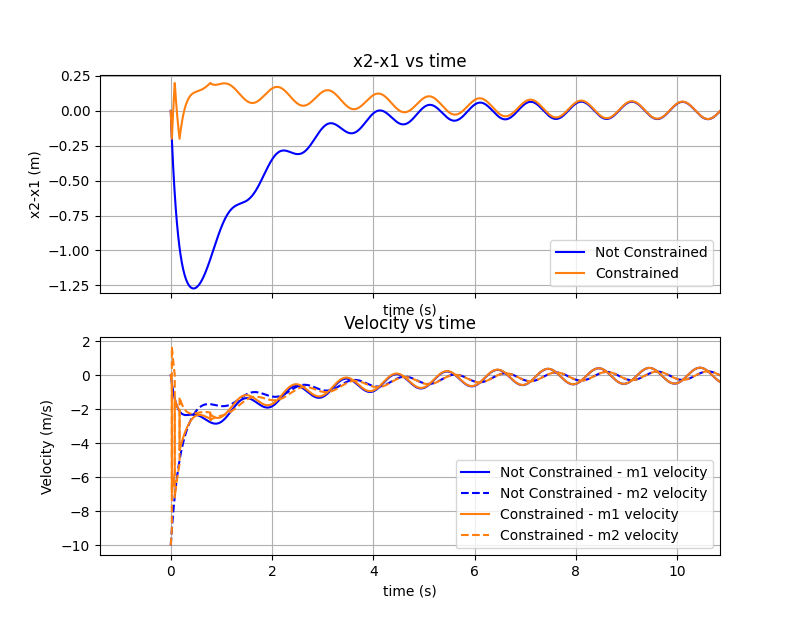
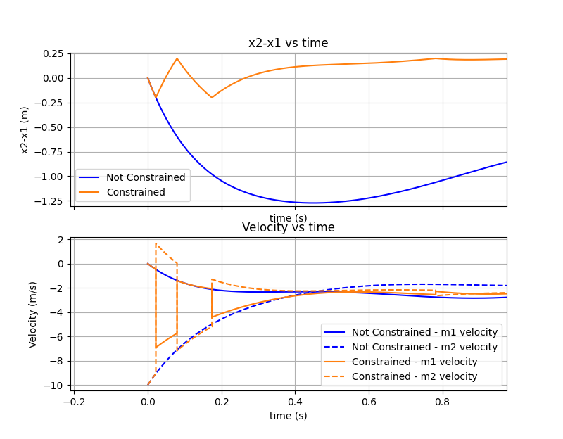
It's cool to see in the constrained case, how the speeds reverse and how the simulation shows some banging around of the cars before they settle and start to follow the unconstrained case. I set the limits to be: \(l_{min}=-0.2 \, m,l_{max}=0.2 \, m\). The distance is really a delta length from the resting length.
Conservation of Energy
I wanted to look at the conservation of energy since we are putting energy into the system, removing it via friction and the damper, storing it in the spring, and also have the kinetic energy of the cars. We have for the conservation of energy:
$$ (KE+PE)_o + \int_0^t (Input Energy) dt - \int_0^t (Friction Energy) dt - \int_0^t (Damper Energy) dt = KE(t) + PE(t) $$ $$ (KE+PE)_o + \int_0^t (F_1 \dot{x}_1 + F_2 \dot{x}_2) dt - \int_0^t (f_1 \dot{x}_1 + f_2 \dot{x}_2) dt - \int_0^t c_{12}(\dot{x}_1 - \dot{x}_2)^2 dt $$ $$ = \frac{1}{2}(m_1 \dot{x}_1^2 + m_2 \dot{x}_2^2) + \frac{1}{2} k_{12} (x_1-x_2)^2 $$Looking at the conservation of energy, we can plot all those terms and I can also bring all the terms on the RHS to the LHS so that I have an energy equation that is supposed to equal 0. I show all of this in the plot below using the Dual Time Stepping method for the same conditions as above and the not constrained case:
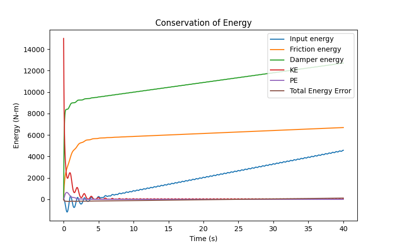
The plot shows high initial KE which we specify and then we quickly dissipate a lot of that energy and put some more energy into the system via the forcing function that is also dissipated using the damper and friction. More energy is dissipated through the damper than friction but the numbers I chose to use are fairly arbitrary so this might not be physically accurate. We do see how the forcing function is relatively weak and any energy we put into the system is dissipated rather quickly.
The energy that the forcing function provides is oscillatory as well. This is because the velocity and the force functions are not perfectly aligned so there is oscillation. The forcing function energy and dissipation energies continuously increase since we are looking a the integral from the beginning. The current energy in the system is a function of the initial energy and history (how much energy has been added and removed).
Below I also show the total energy to see how accurate are we (the closer to 0, the better). The top plot shows total energy which is the equation I have when I bring all terms on the RHS to the LHS from my energy conservation equation. The bottom plot is that same equation but as a percent of the initial energy and input energy.
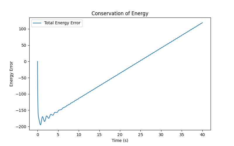
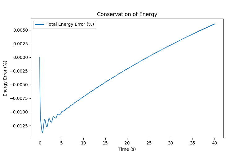
We see that the energy balance is quite close to 0 which is what we expect. There is some error due to the numerical integration. Also this error accumulates when we integrate for the input energy and dissipated energy (through friction and the damper).
Force and Damper Dissipated Energy vs Initial Train Speed
I mentioned this briefly at the beginning but one application of this type of analysis and model is to look at the force the coupling experiences when trains are connecting to each other. One could also consider the total energy dissipated in the damper. I am only looking at the case with two cars and one is moving to connect to the other. For simplicity, I also ignore the geometry constraint that would apply in an actual application.
Below I plot the max. force on the coupling vs initial car speed. I am not applying any forcing function but only give car 2 an initial velocity torwards car 1. I also plot the total energy dissipated in the damper vs car 2 initial velocity.
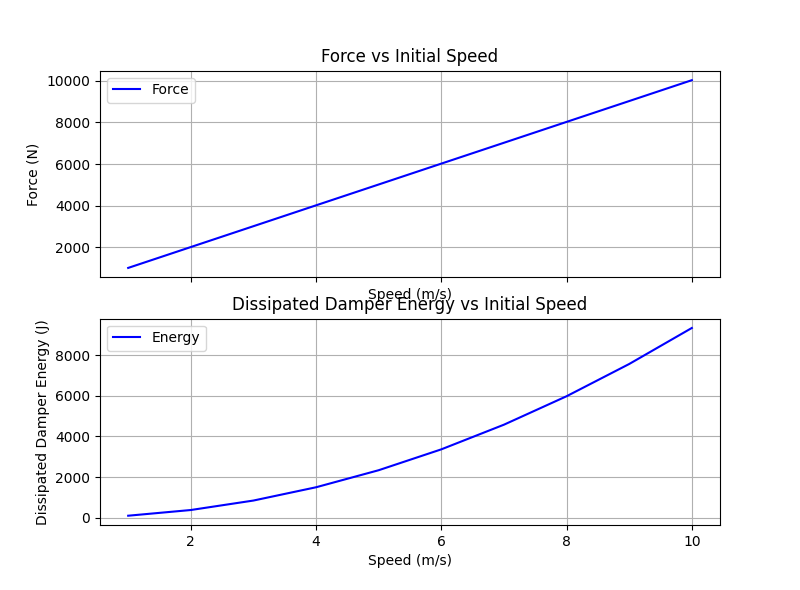
The speeds I looked at are most likely not that realistic but I wanted to use round numbers. 10 m/s would be quite the collision. Also, my other numbers, car mass, spring constant, damper coefficient, friction are mostly made up.
The trends are interesting though. We see a linear function between force and velocity while we have a parabolic like shape between energy and speed.
I won't say more about this but it was interesting to model this and compare several methods. In the end, I could see how using Simscape could be beneficial but also building a better model in Python wouldn't seem like that much of a time/cost investment.