CFD Project

I took an interest in Computational Fluid Dynamics (CFD) mostly because it combines two things I already had interests in: math and fluids. Early in my career, I worked alongside those who did work in reacting flows which takes CFD to a different level and this helped start my interest in modeling.

At GE Aerospace, CFD came back to me when I was working on modeling a fuel system. Typically, with control modeling you use linear models due to their simplicity, ease of use, and that linear control theory is a very established fields. A question that always arises is how valid the models are. Without experimental data (some rigs take a long time to build), a higher fidelity model can be used to help guide some of the simpler models. This is where CFD came in. I built a 1D fluids model to help justify the use of my linear pressure dynamic models. I found the 1D model fun and decided to build a different model here.

The layout of this section will be as follows (click the links to go to a specific section):

1. Introduction: A description of the project, what the tool can do, and some things I learned while doing this
2. Some examples of the tool:
   Example 1: Converging example
   Example 2: Converging-diverging (supersonic) example
   Example 3: Converging-diverging (subsonic) example
   Example 4: Diverging (sonic input) example
   Example 5a: Diverging (subsonic) failed example
   Example 5b: Diverging (subsonic) failed example
   Example 5c: Diverging (subsonic) sort of passed example
3. General Conservation Equations: Derivation of the General Conservation Equations for a Differential Element
4. 1D Equations: Equations used for 1D model (some simplifications and a method for treating area (height) changes along the length of the model)
5. Boundary Conditions: Some notes on boundary conditions (inlet, outlet, and heat input)
6. Solver Information: Description of how model numerically solves equations
7. Future Work: Expansion to 2D

Introduction

The model is essentially a 1D model of a hollow cylinder that can have a changing diameter along the axial direction. The model finds the steady state solution (or abandons the solution if it is taking too long).

The model allows one to input inlet conditions (pressure and temperature are only allowed currently but this can be modified for other properties as the inlet), outlet conditions (pressure), geometry (length, inlet diameter, throat diameter, and outlet diameter). Depending on the configuration (converging, diverging, converging-diverging), the code will pick the correct diameters to use to build the geometry (eventually this will be used in the mesh generation).

Some notes about the conditions the user can input:

• Pressure and temperature inlet conditions might make the most sense physically. Imagine having a source at some pressure and temperature and allowing the fluid to flow through the valve (geometry). You wouldn’t want to specify say pressure and velocity but allow velocity to fall out of the solution
• Pressure as the outlet condition makes sense physically too. You essentially fix the back pressure and allow the fluid to flow (in a way, the back pressure is only fixed far away from the outlet but we ignore this - when we expand to 2D, we can involve this) (the pressure at the outlet is not fixed in reality but will be a function of pressure waves in the geometry)
• When entering the geometry, be mindful that there is symmetry about the axial axis meaning that diameter of the valve is only a function of axial location
• The gas properties can be changed (currently air is used) and the model can be eventually expanded to include real fluids with some modifications needed, particularly in the energy equation (I did this for Hydrogen at GE Aerospace where H2 behaves strangely as a liquid)

Note that in the following examples, some of the solution finding parameters (artificial viscosity coefficient, solution error, number of max. time steps, etc.) were modified for each solution, mainly for visual and time saving reasons. For some solutions, a smaller max. error (used in convergence decisions) can be used to speed up the solution with minimal change to the final steady state solution.

Example 1: Converging solution

Input	Value
Inlet pressure (bar)	1.2
Inlet temperature (deg. C)	100
Outlet pressure (bar)	1
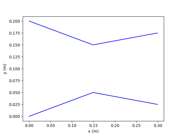
Inlet diameter (m)	0.2
Outlet diameter (m)	0.15
Length (m)	0.3
dx (m/in)	0.001 / ~0.04

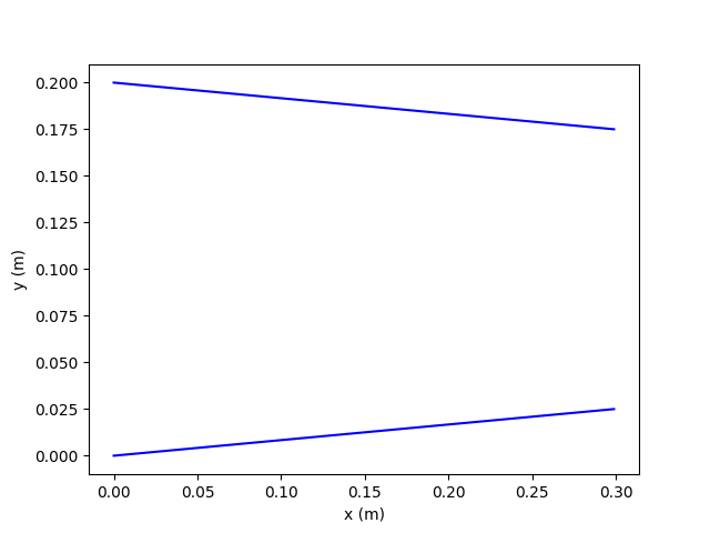
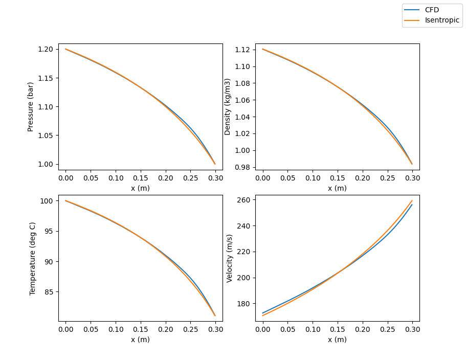
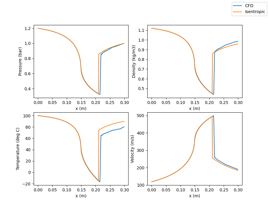
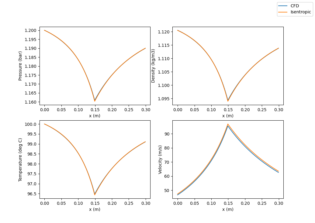
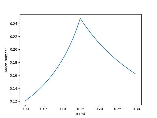
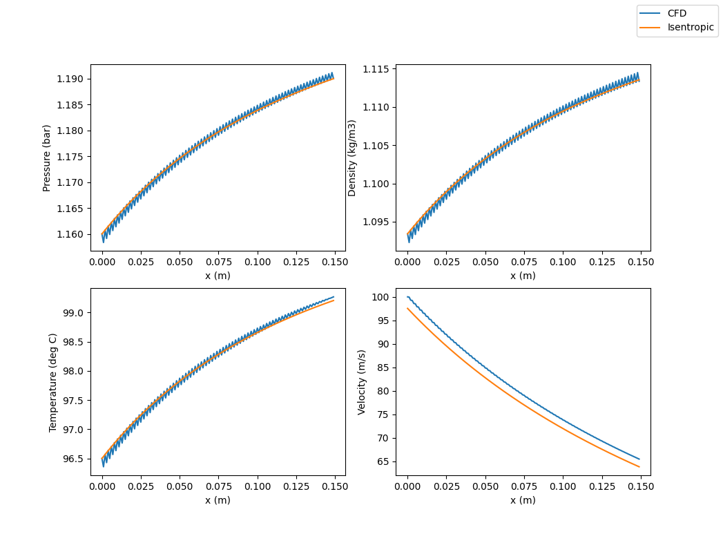
Steady state results show what you would expect, namely, pressure and temperature (and therefore density) dropping as you progress further into the converging section with velocity increasing.

We can compare the CFD result to an isentropic solution using conservation of mass, conservation of momentum, conservation of energy, and the isentropic expansion equations.

Both results give good agreement. The CFD solution (with friction set to 0) should give exact agreement but the artificial friction we add to the solutions (to make them more stable, see discussion further below about CFD model) leads to some slight disagreement.

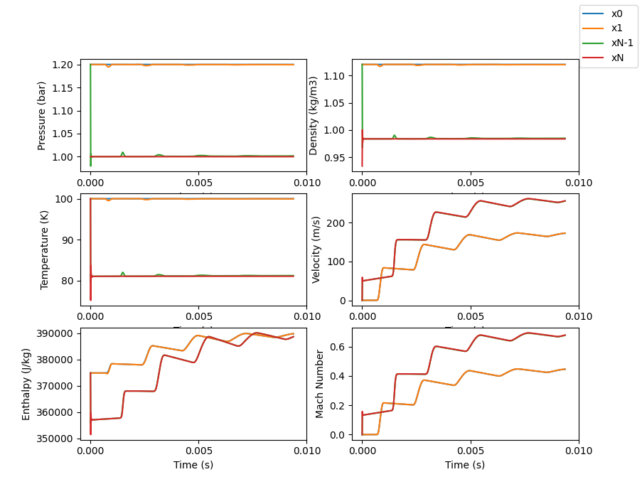
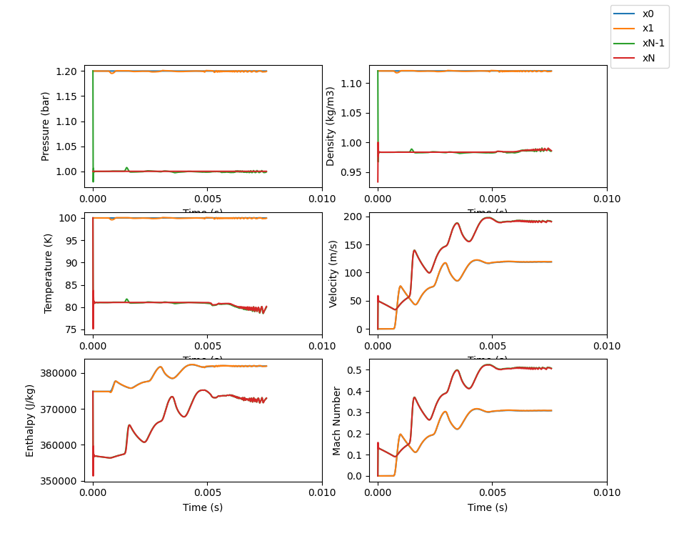
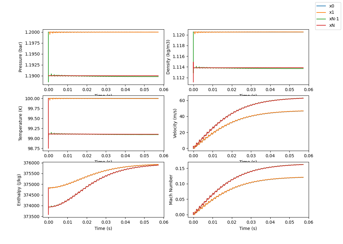
Initial conditions were set to be the same as those at the inlet so for this example, P(x=n)=Inlet Pressure (except for x=N) and the same for the temperature.

The time based results show how the pressure and temperature quickly converge to their correct values while the velocity takes a little longer (which is expected since the initial velocity was set to 0).

The plots also show enthalpy which we expect to be constant since energy is conserved and we are not including any heat addition (this can be added and will be in a different example) or heat losses. The plots shows that the enthalpy at the inlet and the exit converges to the same value.

Our Mach number plot follows the same pattern as the velocity plot.

This time based plot could be representative of a system where one has a converging valve with the outlet of the valve closed, and then instantly opens the valve (no dynamic with the valve opening).

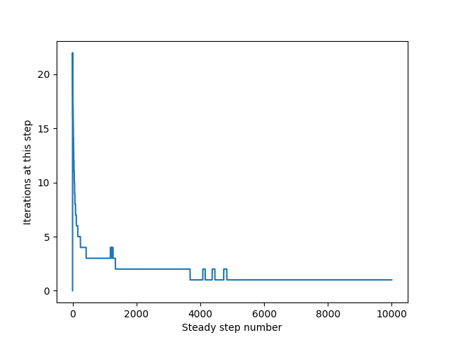
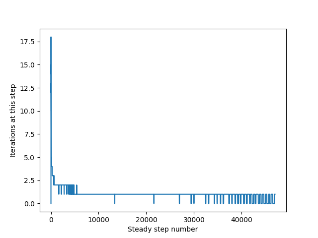
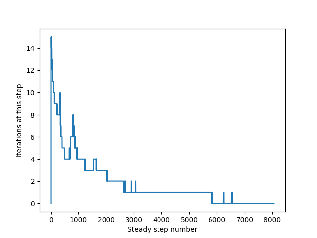
One last plot that could be interesting to look at is the number of iterations the model is going through at each time step. As explained below, the model is a semi-implicit model that iterates at each time step until an acceptable error is reached or the max number of iterations is reached. The plot in this example shows that initially the model is doing more iterations but then the number of iterates starts to level out a few iterations each time step. This makes sense that at the beginning of the simulation, the model is doing “more work” trying to find its way to a solution

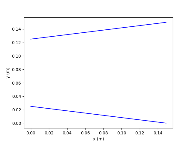
Example 2: Converging-Diverging solution (supersonic)

Input	Value
Inlet pressure (bar)	1.2
Inlet temperature (deg. C)	100
Outlet pressure (bar)	1
Inlet diameter (m)	0.2
Throat diameter (m)	0.1
Outlet diameter (m)	0.15
Length (m)	0.3
dx (m/in)	0.001 / ~0.04

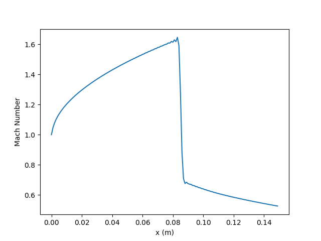
Steady state results show what you would expect, namely, pressure and temperature (and therefore density) dropping as you progress further into the converging section with velocity increasing. At the throat, flow is choked and then supersonic in the diverging section until the shock (including artificial viscosity is key to capturing the shock, without it the solution starts to grow and oscillate around the shock leading to the model crashing.

We can compare the CFD result to an isentropic solution using conservation of mass, conservation of momentum, conservation of energy, and the isentropic expansion equations. Across the shock, we assume negligible shock width so that mass, momentum, and energy are conserved with no friction.

Both results give good agreement. We see a bit of a temperature error between the CFD and Isentropic solutions downstream of the shock. Perhaps the artificial viscosity resulted in a loss of energy somehow. The artificial viscosity term used was an empirical relationship I found that seemed to do well but we can see that it can result in some error depending on its use.

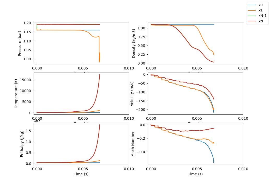
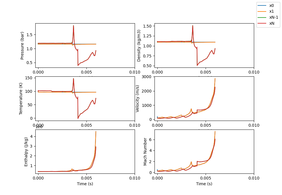
Initial conditions were set to be the same as those at the inlet so for this example, P(x=n)=Inlet Pressure (except for x=N) and the same for the temperature.

The time based results show how the pressure and temperature quickly converge to their correct values while the velocity takes a little longer (which is expected since initial velocity was set to 0)

The plots also show enthalpy which we expect to be constant since energy is conserved but since we observed a difference between the CFD and Isentropic temperature curves in the steady state result, it’s not surprising that the enthalpy at the inlet and outlet don’t converge. The enthalpy difference is about 10,00 J/kg and the temperature difference in the steady state plot was about 10 deg C. Approximating cp of air to be 1,000 J/kg/K and the difference seems to be explained by that temperature difference in the steady state response.

Our Mach number plot follows the same pattern as the velocity plot.

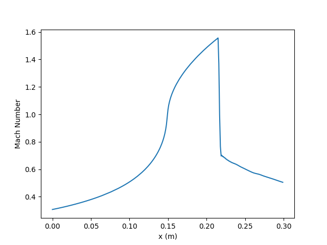
With the converging-diverging valve and a shock in the diverging section, we expect the throat to be choked. Looking at the Mach number steady state result at x = 0.15 m, we see that M is about 1 at that point. It’s also interesting to note that dM/dx is very high near the throat while it starts to taper off before the shock. The sharp decrease in M just beyond x = 0.20 m is the shock. The shock almost acts as a discontinuity as the velocity, pressure, and temperature are much different on each side of the shock

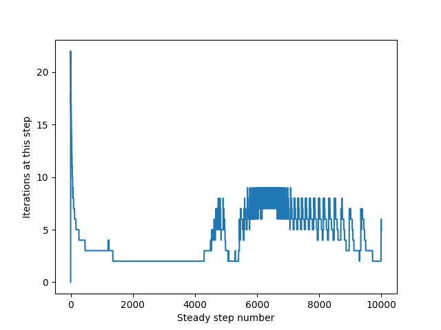
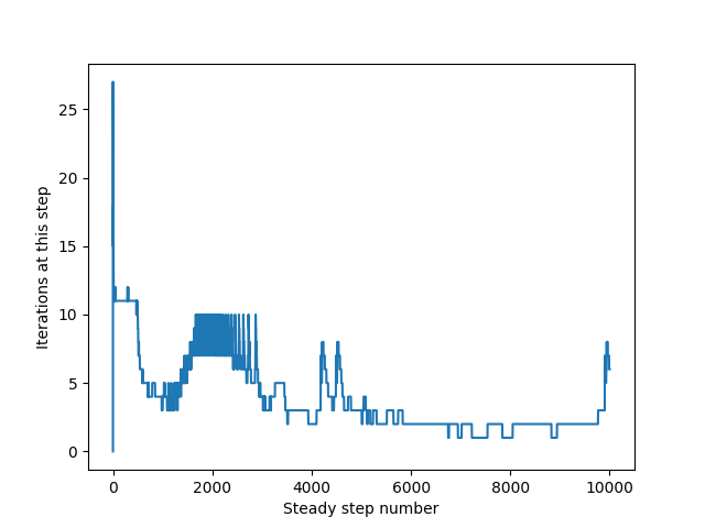
Similar to the converging solution above, we can look at the number of iterations at each time step. Not surprising that the converging-diverging solution has many more iterations at each time step. This is probably due to the more complex fluid solution compared to the converging case.

Example 3: Converging-Diverging solution (subsonic)

Input	Value
Inlet pressure (bar)	1.2
Inlet temperature (deg. C)	100
Outlet pressure (bar)	1.19
Inlet diameter (m)	0.2
Throat diameter (m)	0.1
Outlet diameter (m)	0.15
Length (m)	0.3
dx (m/in)	0.001 / ~0.04

Steady state results show what you would expect for a subsonic case, namely, pressure and temperature (and therefore density) dropping as you progress further into the converging section with velocity increasing. In the diverging section, the pressure starts to increase as the velocity starts to decrease. Temperature also starts to increase to conserve energy.

We can compare the CFD result to an isentropic solution using conservation of mass, conservation of momentum, conservation of energy, and the isentropic expansion equations. Across the shock, we assume negligible shock width so that mass, momentum, and energy are conserved with no friction.

Both results give good agreement with isentropic solution almost completely covering the CFD curves.

Interestingly, the time based plots (right) show that this case takes much longer compared to the other examples to reach a steady state value. This is probably due to the smaller pressure difference between inlet and outlet, and therefore the smaller velocities with this example slow down the transfer of momentum and energy.

We see that the velocity at the outlet reaches a higher velocity than the inlet which makes sense since we specified a higher pressure at the inlet then the outlet.

We also see that the enthalpy at the inlet and outlet converge to the same value. Little wiggles in enthalpy and velocity could be due to pressure waves traveling back and forth. We would need to look at more pressure curves and could also look at pressure vs x (for different time steps close to each other) to evaluate how pressure waves could be going back and forth in the geometry.

Our Mach number plot (Mach number vs x on left) shows how the Mach number still peaks at the throat which is expected since that is the point where the velocity is the lowest.

The outlet area is smaller than the inlet velocity so we have a higher velocity at the outlet compared to the inlet.

Our Mach number curve is very smooth with sharp increases and decreases near the peak at the throat.

Looking at our number of iterations per step (right), we see initially a high number of iterations but it quickly drops and levels off to only around a 2 iterations per step. In future iterations of the code, we could force the code to do at least “x” iterations per step to help make the code more accurate or tighten our error tolerance.

For this example, it looks like our error tolerance is sufficient.

Example 4: Diverging Example (sonic input)

With the diverging geometry, the code is set up to allow a sonic input boundary where all properties (including velocity) are specified. The velocity is simply the speed of sound at the specified temperature.

Input	Value
Inlet pressure (bar)	0.7
Inlet temperature (deg. C)	40
Outlet pressure (bar)	1.0
Inlet diameter (m)	0.1
Outlet diameter (m)	0.15
Length (m)	0.15
dx (m/in)	0.001 / ~0.04

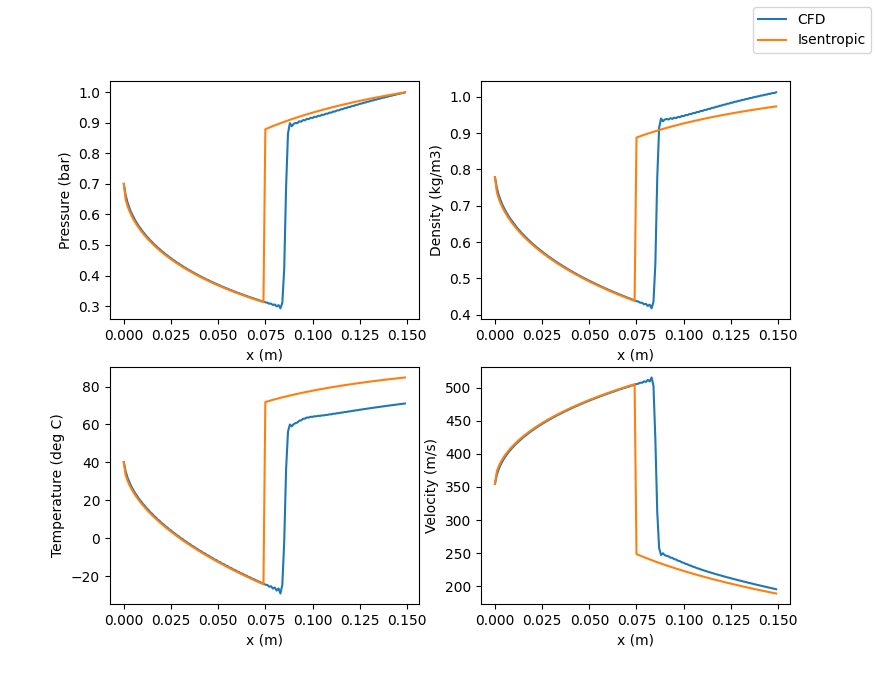
Steady state results show similar results to the diverging section in Example 2. This is what we expected since we selected a sonic input meaning that the boundary condition at the inlet is fully specified (pressure, temperature, velocity).

We see some error between the CFD and Isentropic solutions. This could be due to the dx resolution and/or the artificial viscosity. We would need to do more evaluation before seeing what causes this deviation. The shock location is “off” and this most likely results in the pressure, density, and velocity differences downstream of the shock since the shock “inlet” conditions will be different.

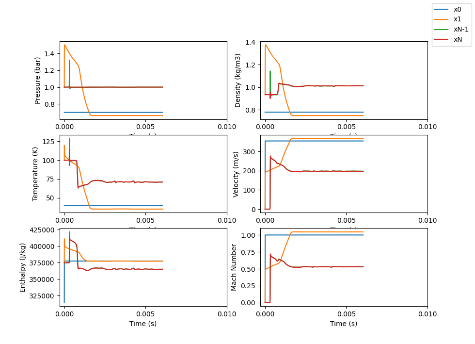
The time based results on the right show that results converge to their steady state values fairly fast (similar response time to Example 2).

We also see our difference again the enthalpy. Enthalpy should be conserved throughout the geometry but our results show it is not. This is again probably due to the artificial viscosity, or at least that could be a first suspect.

Our Mach number plot shows how the flow is choked at the inlet (which we specify) and that the Mach number continues to increase in the diverging section upstream of the shock. After the shock the flow is subsonic and decreases like we would expect in the diverging section of a nozzle.

Comparing to the convergent-divergent geometry (example 2), the result here looks almost identical to the diverging section of the converging-diverging solution which is what we expect (similar shock location and similar Mach number behavior upstream and downstream of the shock).

We see that the diverging solution required more iterations per time step than the previous subsonic examples. The flow field of the sonic diverging example here is a little more complex than a subsonic case and this can be seen in the increased number of iterations per time step.

Example 5a: Diverging solution (no solution found)

In this example, we are looking for the diverging section solution for the subsonic case. In addition to our inputs listed below, we also have our initial velocity set to 0 throughout the geometry. The solution fails to converge.

Input	Value
Inlet pressure (bar)	1.16
Inlet temperature (deg. C)	96.5
Outlet pressure (bar)	1.19
Inlet diameter (m)	0.1
Outlet diameter (m)	0.15
Length (m)	0.15
dx (m/in)	0.001 / ~0.04

The solution for Example 5a fails to converge so we will only look at the time based plot and explain a little why it failed.

Setting the initial velocity to 0 resulted in the model trying to find a solution to a converging geometry with the wrong boundary conditions. We specify the inlet conditions (2 properties and let velocity float) and only specify one outlet property. This leads to an unstable solution and the solution starts to grow uncontrollably (see the temperature curve for the outlet - in the converging example, the temperature needs to be specified at the inlet).

You can see how the model starts to say the velocity should be negative since the flow is going from high pressure to low pressure. We are trying to recreate the subsonic diverging section result from the converging-diverging valve but having the velocity initially set to 0 makes this impossible. It’s hard to imagine physically this initial set up resulting in the desired solution.

Example 5a: Diverging solution (no solution found)

In this example, we are looking for the diverging section solution for the subsonic case. In addition to our inputs listed below, we also have our initial velocity set to 100 throughout the geometry. The solution fails to converge.

Input	Value
Inlet pressure (bar)	1.16
Inlet temperature (deg. C)	96.5
Outlet pressure (bar)	1.19
Inlet diameter (m)	0.1
Outlet diameter (m)	0.15
Length (m)	0.15
dx (m/in)	0.001 / ~0.04

The solution for Example 5b fails to converge so we will only look at the time based plot and explain a little why it failed.

We set the initial velocity to 100 m/s to help the solution converge on the solution we wanted to find. We see instead that the solution started to grow uncontrollably and failed to find a solution. We see that the velocity actually continues to increase meaning that the velocity at the inlet continued to increase past choked flow and became supersonic. With the way we are finding a solution to the problem, this cannot be handled by the equations and the numerical solver. At choked or above, the velocity must be specified at the inlet and cannot be allowed to float.

You can start to see how difficult it can be to find a solution to the subsonic diverging section. The initial conditions need to be specified really well. Our model is currently useful for finding steady state solutions so for finding diverging geometry subsection solutions, our model is not very useful unless one wants to dedicate a lot of time to trial and error.

Example 5c: Diverging solution (solution found (sort of))

In this example, we are looking for the diverging section solution for the subsonic case. In addition to our inputs listed below, we also specify the inlet velocity to be 100 m/s which is approximately what we find in the throat for the converging-diverging solution. This is not valid to do but we do find a solution with this method.

Input	Value
Inlet pressure (bar)	1.16
Inlet temperature (deg. C)	96.5
Outlet pressure (bar)	1.19
Inlet diameter (m)	0.1
Outlet diameter (m)	0.15
Length (m)	0.15
dx (m/in)	0.001 / ~0.04

We see that specifying the inlet velocity results in a solution that is in agreement with the Isentropic solution.

However, we do see a lot of small oscillations in the pressure, density, and temperature. This is most likely due to the solution being unstable numerically even though the physical solution is stable (or at least we understand the physical solution to physically possible). The reason the solution is not numerically stable is because of the way we specify the inlet boundary condition. The mathematical reasoning is a little messy but it boils down to only specifying two inlet boundary conditions and letting the third float when the boundary condition is subsonic. Three boundary conditions must be specified when the boundary condition is sonic. This comes from the sqrt(1-M^2) term that can be found in the equations (with some modifications) and looking at the characteristic lines.

In this case, we were able to sort of force the solution to work with some luck.

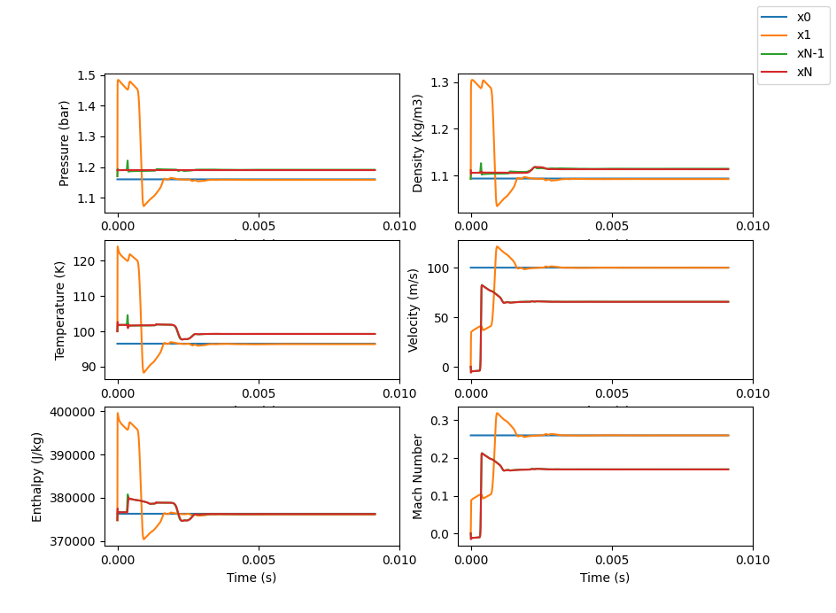
The time based plots show a fast convergence to their steady state values similar to what the converging-diverging example shows.

We see that the input velocity (velocity at x0) is constant as we specify this but the flow is not choked at this point so this is not a valid solution and this approach should not be used (only used here to illustrate it).

It is hard to see where the oscillations in the steady state solution come from in the time based plots. We would maybe have to look at more points but it looks like each node settles to its own steady state solution but there are still oscillations in space (compared to time).

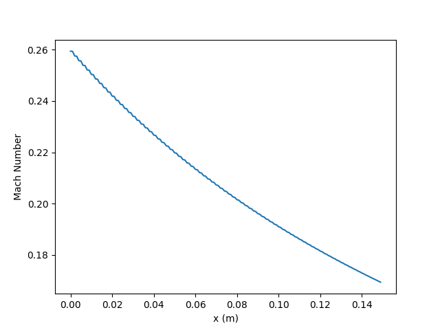
We still see oscillations in space in the Mach number plot on the left. They seem to die out a little as we reach the far boundary condition which could make sense as we move away from the boundary condition where we made an invalid move specifying the inlet velocity.

The Mach number decreases throughout the diverging section which is what we expect in the subsonic diverging case. It would be interesting to see if we put this solution in as an initial condition to the model with no inlet velocity specified and see if it returns the steady state solution we expect. The model is not currently setup to take this kind of initial conditions (the model can only take in uniform initial conditions limiting our capabilities) but it would be interesting to expand to this.

We see that the model doesn’t require many iterations per time step which could be a little surprising. We could expect more iterations since the solution is not numerically stable but it seems the model handled our invalid setup quite well.

General Conservation Equations Derivation

We will derive the conservation equations for the general 3D case. In the next section, we will look at the 1D case which we used to build the model for the examples above. We conduct our derivations assuming we are looking at a control volume in space that is not moving with the fluid so we have fluid moving in and out of our control volume. Compare this to deriving the equation by following a fluid parcel as it moves through space. For all details in the derivation, reference the pdf at the top of this page.

We can start with the general conservation equations, and make simplifications after understanding the general case. Looking at the general case allows us to get comfortable with the equations and the terms and how to translate a physical process into mathematical relations. We will take the infinitesimal volume approach and consider our reference frame to be stationary with respect to the fluid (e.g., control volume is not traveling with a fluid parcel but our reference frame is such that the fluid is passing through the our control volume). First, we look at the conservation of mass.

With the conservation of mass, we have that the change of mass in the control volume is equal to the sum of the mass entering the control volume minus the sum of the mass exiting the control volume.

We can write this as a differential equation where we have:

change of mass in volume = mass in - mass out

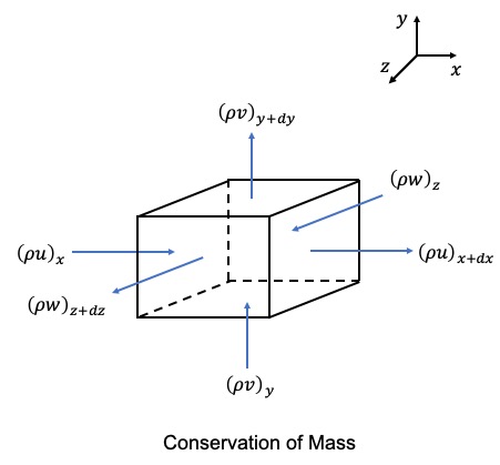
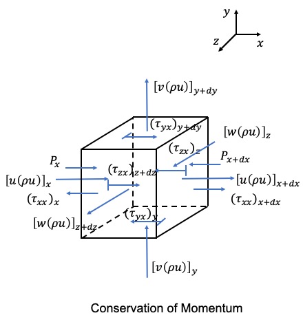
Using the conservation of mass figure, we can start with:

$$\frac{\partial \rho dV}{\partial t} = [(\rho u)_x - (\rho u)_{x+dx}]dydz + [(\rho v)_y - (\rho v)_{y+dy}]dxdz + [(\rho w)_z - (\rho w)_{z+dz}]dxdy$$

Expanding \((\rho u)_{x+dx}\) about x as a Taylor series gives:

$$(\rho u)_{x+dx} = (\rho u)_x + \frac{\partial (\rho u)_x}{\partial x} dx + ...$$

where ... represents higher order terms we neglect

Using a similar approach for the other mass flux terms, we get:

$$\frac{\partial \rho}{\partial t}dxdydz = -\frac{\partial \rho u}{\partial x}dxdydz - \frac{\partial \rho v}{\partial y}dxdydz - \frac{\partial \rho w}{\partial z}dxdydz$$

Simplifying gives:

$$\frac{\partial \rho}{\partial t} = -\frac{\partial \rho u}{\partial x} - \frac{\partial \rho v}{\partial y} - \frac{\partial \rho w}{\partial z}$$

This gives rise to the differential form of the conservaiton of mass:

$$\frac{\partial \rho}{\partial t} = - \nabla \cdot (\rho \vec{U})$$

where \(\vec{U} = (u,v,w)\)

We get the integral form:

$$\int_V \frac{\partial \rho}{\partial t} \, dV = - \int_V \nabla \cdot (\rho \vec{U}) \, dV = \frac{\partial }{\partial t} \int_V \rho \, dV = - \int_S (\rho \vec{U}) \cdot \hat{n} \, dS$$

where \(\hat{n}\) is a unit vector pointing away from the surface

Next, we can look at the conservation of momentum. We’ll only focus on momentum in the x direction but the results are identical for momentum in the y and z directions.

As explained above, we will focus on momentum in the x direction to simplify the explanation. We have that the change of momentum in the control volume in the x direction is equal to the sum of momentum entering and exiting the control volume in the x direction plus the sum of the body and surface forces. Body forces include pressure and any others (such as gravity but we ignore gravity here). Surface forces are mostly viscous forces (e.g., friction).

We can write this as a differential equation where we have:

change of momentum in the x direction = (momentum in - momentum out)x + sum of body forces (in x direction) and sum of viscous forces (in x direction)

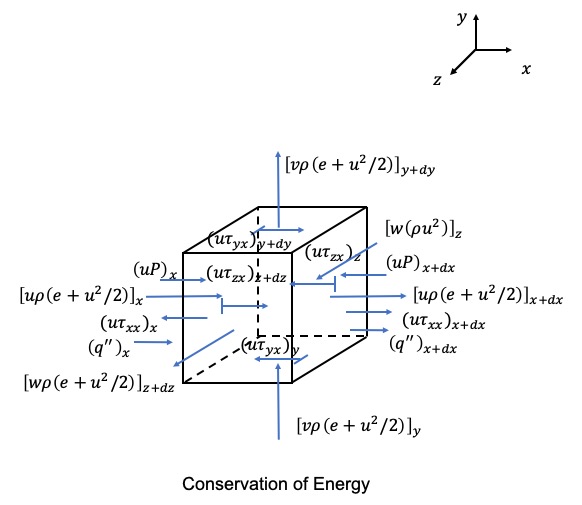
Momentum is directional so we should specify a direction with momentum. We will not do this and instead imply the direction using our velocity components so when we see \(\rho u\), we understand that to be in the x direction. Using the conservation of momentum figure, and only looking at the x component of momentum, we can start with:

$$\frac {\partial (\rho u dV)}{\partial t} = \{[u(\rho u)]_x - [u(\rho u)]_{x+dx}\}dydz + \{[v(\rho u)]_y - [v(\rho u)]_{y+dy}\}dxdz + \{[w(\rho u)]_z - [w(\rho u)]_{z+dz}\}dxdy$$ $$+ [(\tau_{xx})_{x+dx}-(\tau_{xx})_x]dydz + [(\tau_{yx})_{y+dy}-(\tau_{yx})_y]dxdz + [(\tau_{zx})_{z+dz}-(\tau_{zx})_z]dxdy$$ $$ + (P_x - P_{x+dx})dydz$$

\(\tau_{yx}\) is to be understood as the stress on the plane perpendicular to y in the x direction. We can expand the terms using Taylor series, and obtain:

$$\frac {\partial (\rho u)}{\partial t} = - \frac {\partial }{\partial x}[u(\rho u)] - \frac {\partial }{\partial y}[v(\rho u)] - \frac {\partial }{\partial z}[w(\rho u)]$$ $$+ \frac {\partial }{\partial x} \tau_{xx} + \frac {\partial }{\partial y} \tau_{yx} + \frac {\partial }{\partial z} \tau_{zx} - \frac {\partial }{\partial x} P$$

We then get for momentum in the x direction:

$$\frac {\partial (\rho u)}{\partial t} = - \nabla \cdot (\rho u \vec{U}) + \frac {\partial }{\partial x} \tau_{xx} + \frac {\partial }{\partial y} \tau_{yx} + \frac {\partial }{\partial z} \tau_{zx} - \frac {\partial }{\partial x} P$$

and similarly for the y and z directions:

$$\frac {\partial (\rho v)}{\partial t} = - \nabla \cdot (\rho v \vec{U}) + \frac {\partial }{\partial x} \tau_{xy} + \frac {\partial }{\partial y} \tau_{yy} + \frac {\partial }{\partial z} \tau_{zy} - \frac {\partial }{\partial y} P$$ $$\frac {\partial (\rho w)}{\partial t} = - \nabla \cdot (\rho w \vec{U}) + \frac {\partial }{\partial x} \tau_{xz} + \frac {\partial }{\partial y} \tau_{yz} + \frac {\partial }{\partial z} \tau_{zz} - \frac {\partial }{\partial x} P$$

Since momentum is directional, when looking at the differential form of momentum, it's not easy to simply to one equation but we have one equation per direction. For the integral form, we can simply to one direction (with a little handwaving to make it look clean). For this, we can first look at the x component and simply our viscous forces:

$$\frac {\partial (\rho u)}{\partial t} = - \nabla \cdot (\rho u \vec{U}) + \nabla \cdot \sigma_x - \frac {\partial }{\partial x} P$$

where \(\sigma_x = (\tau_{xx}, \tau_{yx}, \tau_{zx})\). We then can integrate around our volume:

$$\int_V \frac {\partial (\rho u)}{\partial t} \, dV = - \int_V \nabla \cdot (\rho u \vec{U}) \, dV + \int_V \nabla \cdot \sigma_x \, dV - \int_V \frac {\partial }{\partial x} P \, dV$$

Using the divergence theorem gives:

$$\int_V \frac {\partial (\rho u)}{\partial t} \, dV = - \int_S \rho u \vec{U} \cdot \hat{n} \, dS + \int_S \sigma_x \cdot \hat{n} \, dS - \int_V \frac {\partial }{\partial x} P \, dV$$

I don't apply the divergence theorem on the P term yet (the reason will become clear). It's also important to point out that for \(\nabla \cdot (\rho u \vec{U})\), we get a scalar and that we know we need a direction for momentum so this term (and terms like it) should have a direction associated with it (in this case, \(\hat{i}\)).

We can integrate for the other directions and obtain:

$$ x\: direction: \int_V \frac {\partial (\rho u)}{\partial t} \, dV = - \int_S \rho u \vec{U} \cdot \hat{n} \, dS + \int_S \sigma_x \cdot \hat{n} \, dS - \int_V \frac {\partial }{\partial x} P \, dV$$ $$ y\: direction: \int_V \frac {\partial (\rho v)}{\partial t} \, dV = - \int_S \rho v \vec{U} \cdot \hat{n} \, dS + \int_S \sigma_y \cdot \hat{n} \, dS - \int_V \frac {\partial }{\partial y} P \, dV$$ $$ z\: direction: \int_V \frac {\partial (\rho w)}{\partial t} \, dV = - \int_S \rho w \vec{U} \cdot \hat{n} \, dS + \int_S \sigma_z \cdot \hat{n} \, dS - \int_V \frac {\partial }{\partial z} P \, dV$$

We can combine all of these to obtain:

$$\int_V \frac {\partial (\rho u + \rho v + \rho w)}{\partial t} \, dV = - \int_S (\rho u \vec{U} \cdot \hat{n} + \rho v \vec{U} \cdot \hat{n} + \rho w \vec{U} \cdot \hat{n}) \, dS$$ $$ + \int_S (\sigma_x \cdot \hat{n} + \sigma_y \cdot \hat{n} + \sigma_z \cdot \hat{n} ) \, dS - \int_V (\frac {\partial }{\partial x} P + \frac {\partial }{\partial y} P + \frac {\partial }{\partial z} P )\, dV$$

which can be simplified down to our integral form:

$$\int_V \frac {\partial (\rho \vec{U})}{\partial t} \, dV = - \int_S (\rho \vec{U} (\vec{U} \cdot \hat{n})) \, dS + \int_S \bar{\sigma} \hat{n} \, dS - \int_S P \hat{n} \, dS$$

Here, \(\bar{\sigma}\) is a matrix representing our viscous forces:

$$\bar{\sigma} = \begin{bmatrix} \tau_{xx} & \tau_{yx} & \tau_{zx} \\ \tau_{xy} & \tau_{yy} & \tau_{zy} \\ \tau_{xz} & \tau_{yz} & \tau_{zz} \end{bmatrix} $$

It's implied but we assume that our velocity vector is a column vector in this analysis. The complete momentum equation should include gravity and other body/surface forces but we neglect these in the derivation as we won't use them in the model.

Next, we can look at the conservation of energy. Energy doesn’t have a direction but for body forces, our assumptions on the directions influences if the work done on the control volume is positive or negative.

For the conservation of energy, we have that the change of energy in the control volume is equal to the sum of the energy entering and leaving the control volume plus the net rate of energy done on the control volume.

The sum of energy entering and leaving is fairly simple. This is similar to the conservation of mass where we have some energy entering the control volume and some leaving. This can also include heat transfer (e.g., conduction captured in the q” term).

The net rate of energy done on the control volume can be a little trickier. We will focus on the work done from pressure and the shear force. We assume that the pressure at x is acting in the positive x direction. The pressure at x+dx is acting in the negative x direction. This leads to the work being done by the pressure at x being positive (work done on the control volume). The work from the pressure at x+dx is negative (work done by the control volume). For the viscous stress, we assume that velocity increases in the positive x, y, and z directions. This means we assume that the velocity in the x direction at y+dy is greater than y. This means that the fluid at y+dy is trying to pull the fluid in the control volume in the x direction. The velocity in the x direction at y is less so this fluid is trying to pull the fluid in the -y direction. In this way, the work done by the viscous stress in the x direction at y+dy is positive (see (u*tau)_(yx) in the figure) compared to the viscous stress at y. We again only show forces and flow in the x direction for simplicity but one can expand what we said above to all directions.

We can write this as a differential equation where we have:

change of energy against time = (energy in - energy out) + sum of work done against control volume + any other heat sources within control volume (we neglect heat sources but they can occur in nature)

change of energy:

$$\frac {\partial \rho (e+|\bar{U}|^2)}{\partial t} \, dV$$

flow of energy in - flow of energy out:

$$\{[u \rho (e+\frac{u^2}{2}+\frac{v^2}{2}+\frac{w^2}{2})]_x - [u \rho (e+\frac{u^2}{2}+\frac{v^2}{2}+\frac{w^2}{2})]_{x+dx}\}dydz $$ $$+ \: \{[v \rho (e+\frac{u^2}{2}+\frac{v^2}{2}+\frac{w^2}{2})]_y - [v \rho (e+\frac{u^2}{2}+\frac{v^2}{2}+\frac{w^2}{2})]_{y+dy}\}dxdz $$ $$+ \: \{[w \rho (e+\frac{u^2}{2}+\frac{v^2}{2}+\frac{w^2}{2})]_z - [w \rho (e+\frac{u^2}{2}+\frac{v^2}{2}+\frac{w^2}{2})]_{z+dz}\}dxdy$$ $$=-\frac{\partial }{\partial x}[u \rho (e+\frac{u^2}{2}+\frac{v^2}{2}+\frac{w^2}{2})]dxdydz-\frac{\partial }{\partial y}[v \rho (e+\frac{u^2}{2}+\frac{v^2}{2}+\frac{w^2}{2})]dxdydz$$ $$-\: \frac{\partial }{\partial z}[w \rho (e+\frac{u^2}{2}+\frac{v^2}{2}+\frac{w^2}{2})]dxdydz$$ $$= \: -\nabla \cdot \bar{U} \rho (e + \frac{u^2+v^2+w^2}{2}) dxdydz = -\nabla \cdot \bar{U} \rho (e + \frac{|\bar{U}|^2}{2}) dxdydz$$

rate of energy by forces:

$$\{[u \tau_{xx} + v \tau_{xy} + w \tau_{xz} - uP]_{x+dx}-[u \tau_{xx} + v \tau_{xy} + w \tau_{xz} - uP]_{x}\}dydz$$ $$+ \: \{[u \tau_{yx} + v \tau_{yy} + w \tau_{yz} - vP]_{y+dy}-[u \tau_{yx} + v \tau_{yy} + w \tau_{yz} - vP]_{y}\}dxdz$$ $$+ \: \{[u \tau_{zx} + v \tau_{zy} + w \tau_{zz} - wP]_{z+dz}-[u \tau_{zx} + v \tau_{zy} + w \tau_{zz} - wP]_{z}\}dxdz$$ $$ = \: \frac{\partial }{\partial x}[u \tau_{xx} + v \tau_{xy} + w \tau_{xz} - uP]dxdydz + \frac{\partial }{\partial y}[u \tau_{yx} + v \tau_{yy} + w \tau_{yz} - vP]dxdydz$$ $$+ \: \frac{\partial }{\partial z}[u \tau_{zx} + v \tau_{zy} + w \tau_{zz} - wP]dxdydz$$ $$ = \: \nabla \cdot \bar{\sigma}^T \bar{U} dV - \nabla \cdot \bar{U}P dV$$

heat transfer:

$$(q_x^"-q_{x+dx}^")dydz + (q_y^"-q_{y+dy}^")dxdz + (q_z^"-q_{z+dz}^")dxdy$$ $$= \: - \frac{\partial q_x^"}{\partial x}dV - \frac{\partial q_y^"}{\partial y}dV - \frac{\partial q_z^"}{\partial z}dV = - \nabla \cdot \bar{q^"} dV$$

where \(\bar{q^"}=(q_x^",q_y^",q_z^")\) and \(q_x^"=-k\frac{\partial T}{\partial x}\) (and similar for the other directions)

Combining everything gives the differential form:

$$\frac {\partial \rho (e+|\bar{U}|^2)}{\partial t} = -\nabla \cdot \bar{U} \rho (e + \frac{|\bar{U}|^2}{2}) + \nabla \cdot \bar{\sigma}^T \bar{U} - \nabla \cdot \bar{U}P - \nabla \cdot \bar{q^"} $$

We can use the divergence theorem directly on the RHS and obtain the integral form:

$$\int_V\frac {\partial \rho (e+|\bar{U}|^2)}{\partial t} \, dV = \int ( - \bar{U} \rho (e + \frac{|\bar{U}|^2}{2}) + \bar{\sigma}^T \bar{U} - \bar{U}P - \bar{q^"} ) \cdot \hat{n} \, dS$$

I use the differential form for the derivation. We’ll see below but I also use the differential form for implementing the 1D conservation equations in the model. The integral form has some advantages (e.g., easier to handle complex geometries, easier to capture discontinuities, more flexibility with numerical techniques) when implementing the equations into a model but we will focus on the differential form for now. I find that the differential form is a little easier to understand and derive.

The integral method will be re-visited when we go 2D (but that has not been implemented yet).

1D Conservation Equations Derivation

The examples above are based on a 1D approach that will be explained here. In our general conservation equation derivations, we assumed that the area (dy*dz) when looking in the x direction was constant across the cell. For our 1D model to handle changes in area (symmetrical changes), we need to slightly modify our equations to look at this.

We will follow the same outline as above, first looking at the conservation of mass then momentum then energy. The next section will talk briefly about boundary conditions and the section after that, about how the 1D conservation equations we derive here are solved numerically. We will only look at the differential form in this section.

First we look at the conservation of mass. We see that it is quite similar to the conservation of mass schematic we used in the general section above. We note that the area is different at the inlet compared to the outlet but we still have:

change of mass in volume = mass in - mass out

Note that the area is larger at the outlet than the inlet. We could have drawn the schematic with the inlet larger than the outlet and we would get the same result. It will be important to pay attention to this since assumptions on the area change are important in the derivation, particularly in the momentum and energy equations.

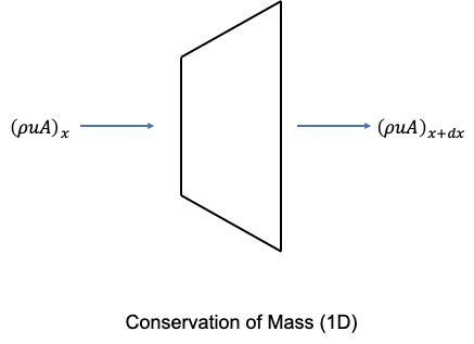
We start with:

$$\frac{\partial \rho dV}{\partial t} = [(\rho A)_x - (\rho u A)_{x+dx}]$$ $$\frac{\partial (\rho A dx)}{\partial t} = -\frac{\partial (\rho u A)}{\partial x}dx$$

Simplifying gives:

$$A \frac{\partial \rho}{\partial t} = -\frac{\partial (\rho u A)}{\partial x}$$

This gives rise to the differential form of the conservaiton of mass:

$$\frac{\partial \rho}{\partial t} = - \frac{1}{A} \frac{\partial (\rho u A)}{\partial x}$$

Next, we look at the conservation of momentum. We note again that it is fairly similar to the general form we had above and it follows the same idea:

change of momentum in the x direction = (momentum in - momentum out)x + sum of body forces (in x direction) and sum of viscous forces (in x direction)

We do have new body forces due to the change in area compared to the general case above. We say that the pressure on this face (slanted face due to the change in area) is the average of the inlet and outlet pressures as shown. This force is acting against the face and we can see that the force from the pressure will be perpendicular to that face. From the symmetry, we see that the forces in the y direction from the top and bottom face will cancel. The force in the x direction is new and we have one part from the top face and a second from the bottom face. From the geometry, we know that the x component is F * cos(pi/2-theta) where cos(pi/2-theta) = sin(theta) and sin(theta) = dA/2 / sqrt(dx^2+(dA/2)^2). We note that our dA is assumed positive so we add this pressure force in the x direction. If we assumed dA was negative, we would be subtracting and also have -dA so we would get the same result.

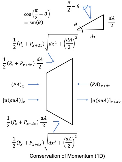
We start with:

$$\frac{\partial \rho u dV}{\partial t} = \{[u(\rho u A)]_x - [u(\rho u A)]_{x+dx}\} + [(PA)_x-(PA)_{x+dx}] + 2\frac{1}{2}(P_x+P_{x+dx})\frac{dA}{2}$$ $$A \frac{\partial (\rho u)}{\partial t}dx = -\frac{\partial [u(\rho u A)]}{\partial x}dx - \frac{\partial PA}{\partial x}dx + PdA + \frac{1}{2} \frac{\partial P}{\partial x}dxdA$$

We simplify and obtain:

$$A \frac{\partial (\rho u)}{\partial t} = -\frac{\partial [u(\rho u A)]}{\partial x} - \frac{\partial PA}{\partial x} + P \frac{dA}{dx} + \frac{1}{2} \frac{\partial P}{\partial x}dA$$

The differential form is then:

$$\frac{\partial (\rho u)}{\partial t} = -\frac{1}{A} \frac{\partial [u(\rho u A)]}{\partial x} - \frac{1}{A} \frac{\partial PA}{\partial x} + P \frac{dA}{dx} + \frac{1}{2} \frac{\partial P}{\partial x} \frac{dA}{A}$$ $$\frac{\partial (\rho u)}{\partial t} = -\frac{1}{A} \frac{\partial [u(\rho u A)]}{\partial x} - \frac{1}{A} \frac{\partial PA}{\partial x} + P \frac{dA}{dx} + \frac{1}{2} \frac{\partial P}{\partial x} d \ln (A)$$

We look at the conservation of energy next. We again follow the same general procedure as for the general case:

change of energy against time = (energy in - energy out) + sum of work done against control volume + any other heat sources within control volume (we neglect heat sources but they can occur in nature)

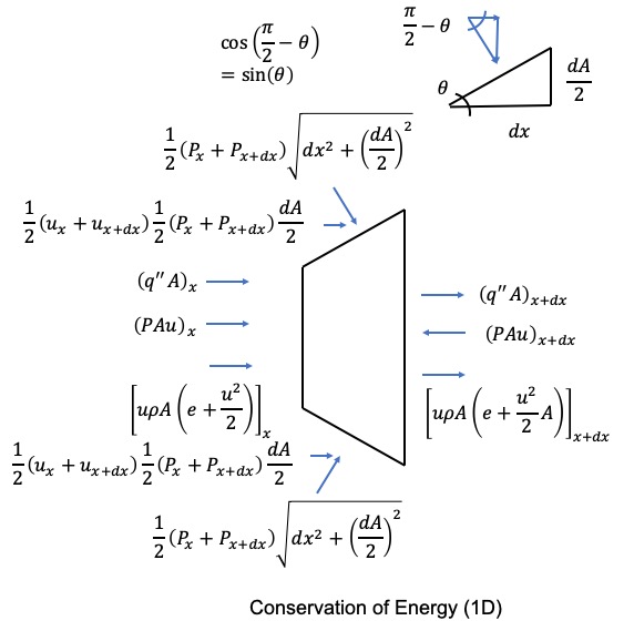
We show in the schematic our new force on the slanted face that we found in the momentum section above for the 1D case. We can then say that we have a new energy term from that force and we can use the average of the inlet and outlet velocity and the force term to get a new energy term as shown in the schematic on the right. THIS IS WRONG.

This is wrong because no fluid is passing through the new slanted face so no work is being done the fluid in the control volume from that force. It is true that the force should be accounted for in the momentum equation since it is a body force that is new because of the changing area (compared to the constant area). However, since no fluid is passing through that surface, there is no work being done on the fluid from that force. This is a situation where one needs to be careful. It can be easy to take the new force in the x direction and then take the average velocity and say there must be a new energy term. This is not correct because physically no flow is coming across that boundary. If we did have flow, then there would be a new energy term.

We still need to modify the energy equation to account for the area change when looking at the body forces and energy flow but we don’t have to add a new term for any extra energy from the different geometry.

We start with:

$$\frac{\partial \rho (e+\frac{u^2}{2}) dV}{\partial t} = \{[u \rho A(e+\frac{u^2}{2})]_x-[u \rho A(e+\frac{u^2}{2})]_{x+dx}\} + [(PAu)_x-(PAu)_{x+dx}]$$ $$ + \: [(q^"A)_x-(q^"A)_{x+dx}] + (u+ \frac{du}{2})(P+ \frac{dP}{2})dA$$

We can use our Taylor series approximation again and obtain:

$$\frac{\partial \rho (e+\frac{u^2}{2})}{\partial t} Adx = -\frac{\partial [u \rho A (e+\frac{u^2}{2})]}{\partial x} dx - \frac{\partial PAu}{\partial x} dx - \frac{\partial q^"A}{\partial x} dx + (u+ \frac{du}{2})(P+ \frac{dP}{2})dA$$ $$\frac{\partial \rho (e+\frac{u^2}{2})}{\partial t} A = -\frac{\partial [u \rho A (e+\frac{u^2}{2})]}{\partial x} - \frac{\partial PAu}{\partial x} - \frac{\partial q^"A}{\partial x} + (u+ \frac{du}{2})(P+ \frac{dP}{2})\frac{dA}{dx}$$

Simplifying this down and neglecting the \(dudPdA, dudA, dPdA\) terms, we obtain:

$$\frac{\partial \rho (e+\frac{u^2}{2})}{\partial t} A = -\frac{\partial [u \rho A (e+\frac{u^2}{2})]}{\partial x} - \frac{\partial PAu}{\partial x} - \frac{\partial q^"A}{\partial x} + uP\frac{dA}{dx}$$

We know have our differential form conservation equations for the 1D case with a changing area (symmetric change). In the next section, we will talk about the boundary conditions and then in the section after that, talk about how we implement the equations and solve them numerically.

Boundary Conditions

Handling boundary conditions is easier for the 1D case compared to 2D or even 3D. The full list of boundary conditions to handle is:

• Inlet conditions
• Outlet conditions
• Wall conditions (flow and thermal/temperature)
• Flow: no slip (velocity equal to 0) or no flow through boundary (V*n=0 where V is velocity vector, n is unit vector perpendicular to surface)
• Thermal/temperature: Constant temperature at wall or heat flux (this could vary)

We will only consider the inlet and outlet conditions. When we go to 2D, we will have to consider the wall boundary conditions. We simplify our approach to the inlet conditions and only allow specifying pressure and temperature (and velocity if the flow is sonic or supersonic). Specifying pressure and temperature is similar to having a constant air supply at some conditions (e.g., ambient temperature at elevated pressure).

Similarly at the outlet, we only specify pressure (if the flow is subsonic at the outlet).

The following schematic illustrates what we specify according to the Mach number at the inlet or outlet:

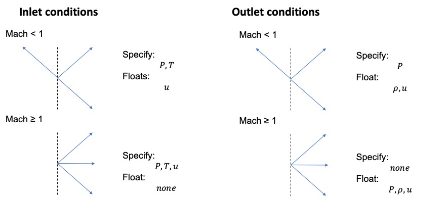
The mathematical reason is a little complex but in the above schematic, we show the characteristic lines for the different mach number conditions at the inlet and the outlet. Essentially, how to specify inlet and outlet boundary conditions simplifies down to the number of characteristic lines entering the control volume. So for example, with a subsonic flow at the inlet, we have two characteristic lines entering the control volume so we specify the pressure and temperature. We could also specify, say density and velocity. We don’t do this because physically, it is easier to understand us having a constant pressure and temperature supply and allowing the velocity to float to match whatever flow is being pulled from our source.

At the outlet with a subsonic flow, we specify pressure only. This makes sense where we have a valve and can control the outlet pressure (e.g., open to ambient conditions).

For the supersonic case, we first need to either specify if the inlet is supersonic or subsonic. In the diverging example above, we specified a sonic inlet for one example to give us the result we want. When the model sees the user specifies a sonic flow at the inlet, the model calculates the sonic velocity based on the inlet temperature and pins the inlet velocity to be sonic. In this case, all inlet conditions are specified.

At the outlet, the model determines based on the velocity and the temperature, if the flow is subsonic or not. If the flow is subsonic, the model uses the pressure boundary condition specified. If the flow becomes supersonic, the model determines that the flow is supersonic and lets all variables at the outlet boundary float.

Solver Information

In this section, I will describe how the solver works. It is a semi-implicit method where the at each time step, the model iterates until some convergence criteria is met. There are weights in the solver that can be modified to make the solution more or less implicit. With a more implicit solution, the error will be smaller but with the increasing number of iterations, the model will take longer to run.

I’ll first modify the equations a bit to make them easier to implement then I will talk about how the solution is found, mainly using the conservation of mass equation as an example.

First, I will start with our 1D equations and simplify them a bit before implementing them. This will save some computation time and make any debugging easier once the code is written.

Starting with the equations in differential form:

$$\frac{\partial \rho}{\partial t}=-\frac{1}{A} \frac{\partial (\rho u A)}{\partial x}$$ $$\frac{\partial (\rho u)}{\partial t} = -\frac{1}{A} \frac{\partial (\rho u^2 A)}{\partial x} - \frac{\partial P}{\partial x}$$ $$\frac{[\rho (e+\frac{u^2}{2})]}{\partial t}=-\frac{1}{A}\frac{\partial[u \rho (e + \frac{u^2}{2})A]}{\partial x} - \frac{1}{A}\frac{\partial (uPA)}{\partial x} - \frac{1}{A}\frac{\partial (q^" A)}{\partial x} + u P \frac{1}{A}\frac{dA}{dx}$$

I refer to the pdf linked at the top of the page for all the details in simplifying the equations. To simplify the momentum equation, we first multiply the conservation of mass equation by \(u\) and then substract that from the conservation of momentum.

The conservation of energy equation can be simplified by multiplying the conservation of momentum equation by u and subtracting from the conservation of energy equation. Then multiply conservation of mass by \(e\) and multiply conservation of mass by \(\frac{u^2}{2}\) and subtract from conservation of energy. We then only consider ideal gasses that obey \(P=\rho R T\).

When we further simplify this, we obtain:

$$\frac{\partial \rho}{\partial t}=-\frac{1}{A} \frac{\partial (\rho u A)}{\partial x}$$ $$\rho\frac{\partial u}{\partial t}=-\rho u \frac{\partial u}{\partial x} - \frac{\partial P}{\partial x}$$ $$c_v \rho \frac{\partial T}{\partial t} = -c_v u \rho \frac{\partial T}{\partial x} - P \frac{\partial u}{\partial x} + k \frac{\partial^2 T}{\partial x^2} - u P \frac{d \ln (A)}{dx} + k \frac{\partial T}{\partial x}\frac{d \ln (A)}{dx}$$

We are now ready to discretize our equations. I will only be showing the momentum equation and using velocity, \(u\), as an example. For more details, refer to the pdf. We consider point \(i\) which is the \(i^{th}\) step in the x direction (\(x_0\) would be the first (e.g., inlet boundary) and \(x_N\) where N-1 is the number of dx increments is the last (e.g., exit boundary)). We look at the Taylor series expansion of velocity at \(i-1\) and \(i+1\):

$$ u_{i-1} = u_i - \frac{d u_i}{dx}dx + \frac{d^2 u_i}{dx^2}\frac{(dx)^2}{2!} - ... + (-1)^n \frac{d^n u_i}{dx^n}\frac{(dx)^n}{n!}$$ $$ u_{i+1} = u_i + \frac{d u_i}{dx}dx + \frac{d^2 u_i}{dx^2}\frac{(dx)^2}{2!} + ... + \frac{d^n u_i}{dx^n}\frac{(dx)^n}{n!}$$

Subtracting the former from the latter gives:

$$ u_{i+1} - u_{i-1} = 2\frac{du_i}{dx}dx+2\frac{d^3 u_i}{dx^3}\frac{(dx)^3}{3!} + 2\frac{d^5 u_i}{dx^5}\frac{(dx)^5}{5!} + ...$$

We then get:

$$ \frac{du_i}{dx} = \frac{u_{i+1}-u_{i-1}}{2dx} - 2\frac{d^3 u_i}{dx^3}\frac{(dx)^2}{3!} - 2\frac{d^5 u_i}{dx^5}\frac{(dx)^4}{5!} + ... = \frac{u_{i+1}-u_{i-1}}{2dx} + O(dx^2)$$

If we add the original equations together, we obtain:

$$ u_{i+1} + u_{i-1} = 2u_i + 2\frac{d^2 u_i}{dx^2}\frac{(dx)^2}{2!} + 2\frac{d^4 u_i}{dx^4}\frac{(dx)^4}{4!} + ...$$

We then get:

$$\frac{d^2 u_i}{dx^2} = \frac{u_{i+1}-2u_i + u_{i-1}}{(dx)^2} - 2\frac{d^4 u_i}{dx^4}\frac{(dx)^4}{4!} - 2\frac{d^6 u_i}{dx^6}\frac{(dx)^6}{6!} - ... = \frac{u_{i+1}-2u_i + u_{i-1}}{(dx)^2} - O(dx^2)$$

We now have a method for discretizing our space derivatives for the first order and second order derivatives. If we neglect the higher order terms, \(dx^2\), we have fairly simple numerical derivatives. For our time derivatives, we use simple forward integration. For the momentum equation, we would obtain the numerical form of:

$$ \frac{u_i^{n+1}-u_i^n}{\Delta t} = -u_i^n \frac{u_{i+1}^n-u_{i-1}^n}{2 \Delta x} - \frac{1}{\rho _i^n}\frac{P_{i+1}^n-P_{i-1}^n}{2 \Delta x}$$

In the above equation, \(i\) is the spatial node and \(n\) is the current time step. The above equation, as is, is an example of an explicit solver where we find the next time step, \(n+1\), based on conditions at the previous time step, \(n\).

We want to modify this (or expand on it) to create an implicit solver. In the implicit solver, the \(n\)s in the above equation are replaced with \(n+1\). This obviously requires some sort of iteration but it results in a much more stable solution. We could have implemented dual time stepping which I believe is a popular method in CFD. I learned about this method after building my own solver so maybe in a future iteration of the model, we can compare the solutions and implement dual time stepping.

My method is based on Picard's method. To find a solution, we first find the time derivative based on the current step. We then find an approximation for the next time using the time derivatives we found at the current step. We then want to find the time derivative again at our approximated next step. We then use weights (X for time derivative found using current step, Y for time derivative found at approximated next step) to find a weighted time derivative. We then keep iterating on our approximated next step until we converge. We use a convergence error term to determine when the solution converges or not. Using the momentum equation again, this is described more below:

To make the solution more stable, we want to first guess (approximate) the values at \(n+1\), and tehn correct by iterating until we find a mostly implicit solution. This method should be called a semi-implicit iterative method since we alter the weights to be more or less implicit.

First we find \(u_i^{n+1}\) by solving the equation below for \(u_i^{n+1}\):

$$ \frac{u_i^{n+1}-u_i^n}{\Delta t} = -u_i^n \frac{u_{i+1}^n-u_{i-1}^n}{2 \Delta x} - \frac{1}{\rho _i^n}\frac{P_{i+1}^n-P_{i-1}^n}{2 \Delta x}$$

We now have an approximation for \(u_i^{n+1}\) and introduce weights \(X,Y\), and iterate. ,We use the weighted average (using the weights) to adjust our approximation of \(u_i^{n+1}\) by solving the following equation for \(u_i^{n+1}\):

$$ \frac{(u_i^{n+1})_N-u_i^n}{\Delta t} = -\frac{Xu_i^n+Y(u_i^{n+1})_{N-1}}{(X+Y)^2} \frac{(Xu_{i+1}^n+Y(u_{i+1}^{n+1})_{N-1})-(Xu_{i-1}^n+Y(u_{i-1}^{n+1})_{N-1})}{2 \Delta x} $$ $$ - \: \frac{1}{X\rho _i^n+Y(\rho _i^{n+1})_{N-1}}\frac{(XP_{i+1}^n+Y(P_{i+1}^{n+1})_{N-1})-(XP_{i-1}^n+Y(P_{i-1}^{n+1})_{N-1})}{2 \Delta x}$$

In the above, our value at \(i+1\) at \(N-1\) is our previous approximation of \(u^{n+1}\) so we have broken up the implicit solution into iterations that improve upon the previous guess. We can limit \(N\) in the code so that the code doesn't get stuck and we introduce a convergence criteria such as \((u_i^{n+1})_N-(u_i^{n+1})_{N-1} < \epsilon \) such that when that inequality holds true, we stop iterating.

The solution should approximate an implicit solution if \(Y>>X\). The same procedure is used for the other two conservation equations. The four variables, \(u,P,\rho,T\) are coupled with each other (with the ideal gas law being used as the fourth relationship) which can slow the solution down but with sufficient weights, the solution should remain stable.

The last thing to mention in this section is that we introduce an artificial viscosity term. This term is needed for the cases where we have a supersonic velocity. Without it, the equations can blow up and become unstable (especially near the shock - one can take the artificial viscosity out of the code and see for themselves - it's difficult to get the solution to be stable without it). The artificial viscosity term is an emperical method I found in a CFD book. I don't know all the details of how it was found and I also forgot to include it in the pdf above (hopefully that is fixed soon). There are some minor (but still very important) details about choosing the time step and spatial step. One much consider the speed of sound and supersonic velocities since that is how information is communicated from node to node so it puts constraints on the spatial and time steps (you can't just choose arbitrarily). With all of these details, one can start to appreciate how CFD may be more of an art that initially thought.

Future Work

There’s a lot to be added to expand our model capabilities. These include (in no particular order):

• Expanding to 2D
• I would like to expand to 2D. To do this, I would compare the finite difference to the finite volume approach. That is basically a comparison between the differential and integral forms. I think the integral form would be easier to implement. If I dedicate the time, I could do both and compare the results to each other.
• I’ll also expand the boundary conditions to play with different wall assumptions. I can also work on implementing more complex geometries. My mesh function will need to be greatly improved. One method for finding solutions to complex geometries is to transform the complex grid into a rectangular grid and solve the rectangular grid transformed problem.
• I can also play with different ways of finding solutions and the right coding language. I used the current model as a way to get familiar with Python but might want to use C++ to improve my C++ skills.
• Expand to include real fluids (this will be similar to what I did in my work at GE when I used the NIST data tables to find my own equations of state at each point).
• Expand to do transient simulations. The model does do a transient simulation technically but only to find the steady state solution. The model can be improved to first find the steady state solution then the user can input changing inlet conditions (or boundary conditions, say a heat flux as a function of time or something else) to see how the fluid reacts. The model can be improved to export a visual showing how conditions change during the solution (could be cool to look at).
• Reacting flows. This would be way down the line but it would be very interesting to first do multi-fluid flows (say air and some liquid) which would introduce new mass conservation equations and alter our momentum and energy equations as well. Then we could add reaction kinetics and solve for reacting flows. Introducing a database of reactions and kinetics, we could see how an air and fuel ignite (or at least predict how they would). We could pick some point and introduce a hot spot by significantly increasing the temperature to kick start the reaction (this would be very cool but will take a long time to build).