Kalman Filter Project

Batteries, in particular Li-Ion batteries, have received a lot of attention due to their high energy densities. This and their long cycle life make them attractive for a variety of applications. One of the challenges with Li-Ion batteries is their relatively flat voltage vs state of charge (SOC) characteristic. Compared to lead batteries, where the dV/dSOC slope magnitude is larger, it’s more difficult to calculate and find the SOC of a Li-Ion battery.

Early in my career, I was working on an energy management project (optimizing batttery charging and discharging using grid and solar power) and this is where I first came across the Kalman filter. During that project, I didn't get to dive into battery SOC esimation technigues too much and this project is motivated by that. I wanted to really understand the Kalman filter and how to apply it.

In this project, I show how to develop an equivalent circuit model of a lithium ion cell. Then I show how the Kalman filter can be derived and implement it using the equivalent circuit model. I compare results to the Coulomb counting method (e.g., current integration). It was a cool experience learning a little bit more about linear algebra and I got look at statistical theory a little bit which sparked a new interest in learning more about probability and statistics.

The layout of this project will be as follows (click the links to go to a specific section):

1. Introduction: A description of the project and the end objective
2. Model (equivalent circuit): Finding the equivalent cricuit model of the lithium ion battery
3. Kalman Filter: Derivation of the Kalman Filter (more specifically the Extended Kalman Filter)
4. Implementation: Implementing the Kalman filter and comparing against Coulomb counting (current integration)
5. Closing Thoughts: Some final thoughts

Introduction

For this project, I was initially looking for a different application for the Kalman filter but the lithium ion application was too good to pass up. One of the big reasons for this was the available data. I’m very grateful for the University of Maryland making this data available: https://calce.umd.edu/battery-data. For this project, I use the first cell available: INR 18650-20R Battery.

When I first started this project, I imagined creating the model would be fairly straightforward but this ended up being the most time consuming part of the project. The Kalman filter relies on a model of the system so the model is obviously a very important and critical part. I had to draw the line somewhere and left some open points on future model development. I was also limited by the data I had and I didn’t fully understand the test setup so I had to make some assumptions that were maybe not valid. After the model development, deriving and implementing the Kalman filter was surprisingly fairly straightforward. The results were a bit mixed where sometimes the Coulomb counting method proved to better match the data than the Kalman filter method. This is where having a poor (or poorer) model can really hurt you and you need to have a method of computing the process and measurement covariance matrices (this is where tuning the Kalman filter becomes important). I didn’t fully optimize the model or filter but showed how the Kalman filter can have benefits over relying purely on a model vs relying purely on measurement (the Kalman filter fuses the two together).

Model (Equivalent Circuit)

Modeling the lithium ion cell as an equivalent circuit has several advantags.

• The equivalent circuit naturally gives a terminal voltage and current
• The circuit must be connected to another network to produce a current
• We can capture the open circuit voltage (OCV) with a voltage source
• We can capture voltage drops and dynamics with resistors and RC circuits, respectively
• It is also fairly intuitive.

In this section, we describe how we build the equivalent circuit model. The Kalman filter relies on having a model of the system. The Kalman filter basically assumes that the system under study is observable and that the measurements we have allow us to estimate/calculate the state, hence the need for a model. The modeling part of the project became more intense than I anticipated and I ended up having to come up a little short on the model (I didn't want to get too carried away and miss my main point with this project). I will only cover the final product. For more details, refer to the pdf.

I'll first look at the basic equations of our model. We have for the voltages:

$$ V = V_{OCV}(SOC) - V_0 - V_1 - V_2 $$ $$ V_{OCV} = V_{OCV}(SOC) \: \: (function \, of \, SOC) $$ $$ V_0 = iR_0$$ $$ \frac{dV_i}{dt} = -\frac{V_i}{R_i C_i} + \frac{i}{C_i} (i = 1,2) $$

For the SOC, we have:

$$ \frac{dSOC}{dt} = -\frac{i}{3600 \, Q} $$

We have \(Q\) is our nominal cell voltage capacity in Ah so we have the 3600 factor to go from hours to seconds. In the above, our current is positive when going out of the cell (discharging) and the sign convention for the voltage and SOC follows.

I'll say more about the equations when we use them in the Kalman filter. We can see they are fairly straightforward. We can solve the RC circuit analytically easily and we will use this in the Kalman filter.

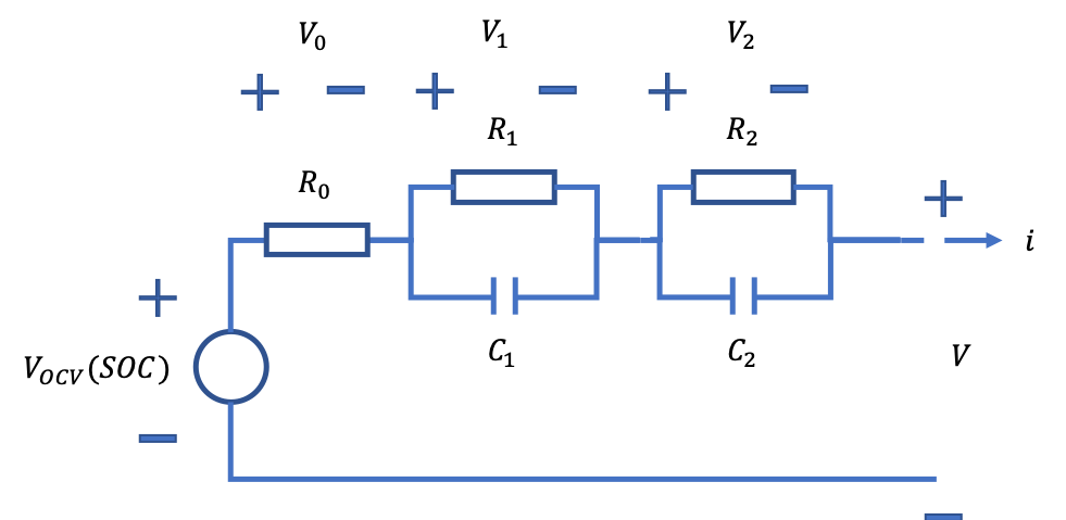
The equivalent circuit model of the lithium ion cell is shown on the right. It's important to note the sign convention implied with the schematic. I show that the current is positive when the cell is discharging (in hindsight, maybe having positive current when the cell is charging would have made more sense).

I then show that we have a voltage source which represents the open circuit voltage (OCV) of the cell. This is the voltage of the cell when no load is applied (e.g., no current being drawn from the cell). It is assumed that this voltage is a function of the state of charge (SOC) of the cell. One can argue that the OCV is also a function of temperature and maybe some other parameters as well (for simplicity, I assume OCV = OCV(SOC) only). I then have a resistor which represents the terminal voltage change when a current is applied. The resistor includes no dynamics so this represents the instantaneous voltage change when the current is changed. I then include two RC circuits to capture internal cell dynamics. I include two to capture "slow" and "fast" dynamics. Through some of the modeling, it became apparent that this might not be necessary and could over complicate the model.

I first found the OCV vs SOC relationship and then found the values for \(R_0,R_1,C_1,R_2,C_2\). I'll first describe how I found the OCV vs SOC relationship.

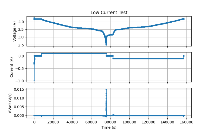
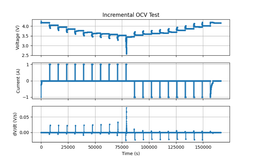
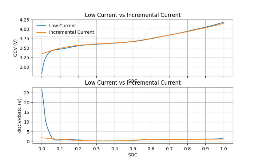
There were two tests I used to explore finding the OCV vs SOC data. The first was a Low Current test where it is assumed that the current is low enough and constant enough that the terminal voltage is approximately the same as the OCV voltage. This test is the first (top) figure on the right. In all the data sets, there is a charge (and discharge) capacity parameter. I use this to find the SOC. I'm not exactly sure how that parameter is measured by I use that for my SOC calculation. Voltage is the terminal voltage and current is the current applied to the cell. For more info, refer to the pdf. The other test is an Incremental Current test where a (higher) current is applied to the cell for a short increment. The cell is allowed to relax and settle between current increments. One can fit a OCV vs SOC curve using the increments then. This test is the second figure on the right.

Finding the OCV vs SOC relationship is fairly straightforward after that. There is data for three different temperatures available (0, 25, and 45 deg. C) and for two samples (1,2). Not all the data is available (you can download it all but some of the data seems to be missing).

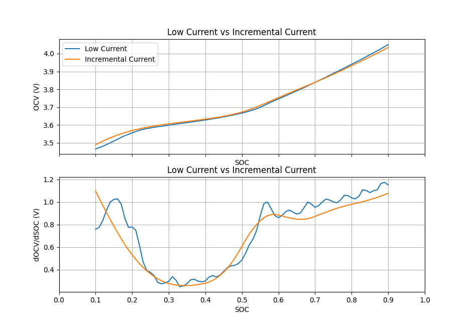
On the right, I show the OCV vs SOC relationship from the Low Current test and the Incremental Current test. I also show dOCV/dSOC which I can calculate from the OCV vs SOC relationship. The dOCV/dSOC curve is important for the Kalman filter (which will be described more below). On the second plot on the right, I show the same but with a trimmed x axis to make the comparison easier. At low SOC, the OCV drops rapidly from the Low Current tests. The impact from the cell dynamics become very significant at low SOC. This is part of the reason why I chose to use the OCV vs SOC relationship from the Incremental Current test.

I will also mention that while there is a (small) temperature dependence on the OCV vs SOC relationship (the curves shown are the average for all temperatures and samples available), I chose to ignore this in the model. I didn't ignore this when looking at the parameters \(R_0,R_1,C_1,R_2,C_2\). From the significant change in OCV vs SOC at low SOC from the Low Current test to the Incremental Current test, one could argue that the parameters, \(R_0,R_1,C_1,R_2,C_2\), should be function of SOC. I did ignore this but discuss it briefly in the pdf.

I won't go into a ton of detail on how I found the parameters but I ended up using Dynamic Stress Test (DST) data to fit the parameters. The DST data subjects the cell to a varying current which really captures the dynamic response of the cell. I use the OCV vs SOC relationship to subtract out the OCV (voltage source in equivalent circuit model). I ended up finding the best fit using the least squares approach.

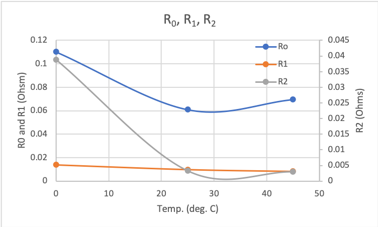
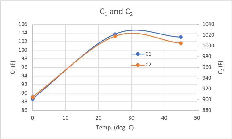
The parameters are shown in plots on the right. The first plot shows the resistance values and the second plot shows the capacitance values. Here, I did find a fairly significant difference depending on the temperature. I think I could make a lot of improvements in finding better parameters but I stopped once I got a fairly suitable model.

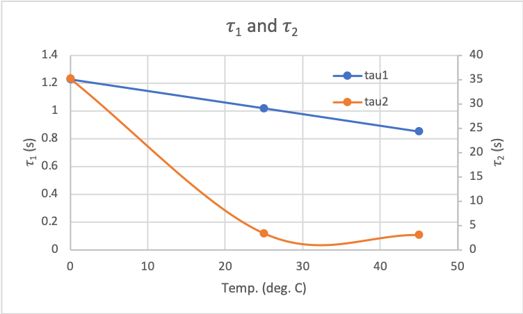
On the right, I show a comparison of the RC circuit time constants. I was able to find a fast time constant (on order of 0.1 seconds) and slower time constant (two orders of magnitude slower). This does suggest that having a fast and slow RC circuit was somewhat valid. It would be interesting to really dive into the physics of the lithium ion cell to understand the driving mechanisms.

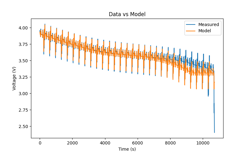
I also show a comparison of the model and the actual terminal voltage for one of the DST data sets (at 25 deg. C starting at 80 % SOC). The model gives fairly good agreement with the actual data except at low SOCs. I discussed this earlier but the dynamcis become very apparement at low SOC. I would have liked exploring how the parameters could vary with SOC but I didn't get to this. This is a common mismatch between the model and the data.

Kalman Filter

In this section, I will walk through the Kalman filter derivation. I won't walk through all the details but all the details are included in the pdf at the top of the page. I will also add that the pdf doens't cover everything and that there are much better derivations and discussions of the Kalman filter online. I will highlight the main pieces of the Kalman filter shown in the diagram below:

We first start with our state equations. We are technically deriving the Extended Kalman Filter. The Kalman Filter is for linear systems and we don't exactly have a linear system so we linearize our non-linear system. This brings us to the Extended Kalman Filter.

Our state and measurement equation are shown below:

$$\dot{x}_k = f_x(x_k) + b_u(u_k) + w_k$$ $$z_k = h(x_k) + b_y(u_k) + v_k$$

Here, we have that \(f_x(x)\) is a nonlinear function of the state, \(x\), \(b_u(u)\) is a nonlinear function of the control input, \(u\), \(h(x)\) is a nonlinear function of the state x,and \(b_y(u)\) is a nonlinear function of the control input, \(u\). For the Kalman filter, not all of the nonlinear functions are actually nonlinear but for now, we assume the general case.

We also have \(w_k\) and \(v_k\). These are the process and measurement noise, respectively. We assume a known standard deviation with zero mean for the noise terms.

One of the first things we have to do is get the state equation into a different form. There are multiple ways of doing this and the simplest may be forward Euler integration where we have \(\dot{x}_k = \frac{x_{k-1}-x_{k}}{\Delta t}\). We will explore two ways when implementing the Kalman filter to the lithium ion SOC application but for now we assume we have:

$$x_{k} = f_x(x_{k-1}) + b_u(u_{k-1}) + w_k$$ $$z_k = h(x_k) + b_y(u_k) + v_k$$

The first part of the Kalman filter is the prediction step. We use the process (state) equation to get our first prediction. You can see how this step is very dependent on the model we have.

We first assume that we have for our initial conditions, an estimate of the state \((x_0 \:or\: x_{k-1}^a)\). We will use \(x_{k-1}^a\) in our derivation. We also assume that we have an initial estimate of the error covariance matrix \((P_o \:or\: P_{k-1})\).

We use the state equation to get:

$$x_k^f = f_x(x_{k-1}^a) + b_u(u_{k-1})$$

Here, \(x_{k-1}^a\) our best estimate of the previous state (eventual output of the Kalman filter). We assume that we know the previous control input \(u_{k-1}\). We also call \(x_k^f\) the forecast state.

We then can find the error of the forecast and take the expected value. We then obtain:

$$ P_k^f = FP_{k-1}F^T + Q_k $$ $$ F = \frac{df_x(x_{k-1}^a)}{dx} $$

You can see our linearization in the \(F\) term. The term, \(Q_k\) represents the process noise covariance term. I have a subscript \(k\) to show that this term can change depending on the state but for our lithium ion application, we will hold that term constant. In our general case for the derivation, \(F\) is a row vector, \(1 \times n\), and \(P\) and \(Q\) are \(n \times n \).

This completes the prediction step part of the Kalman filter.

We first assume that our estimate using the Kalman filter will be:

$$x_k^a = a + K_k z_k$$

In the above, \(x_k^a\) is our estimate of the state using the Kalman filter, \(a\) is a term we want to find, and \(K_k\) is our Kalman gain. We are assuming that the state is a linear combination of \(a\) and our measurement \(z_k\).

To find \(a\), we want our expected error of the esimate to be zero so we find our expected error and solve for \(a\). When we do this, we obtain:

$$a = x_k^f - K_k[h(x_k^f+b_y(u_k))] $$

We then have:

$$ x_k^a = x_k^f + K_k[z_k-h(x_k^f-b_y(u_k))] $$

We are now ready to find the Kalman gain. We plug this back into our error equation. We can then calculate our error covariance matrix, \(P\), again. We then have:

$$ P_k = P_k^f - P_k^f H^T K_k^T - K_k H P_k^f + K_k H P_k^f H^T K_k^T + K_k R_k K_k^T $$

In the above, \(H=\frac{dh(x_k^f)}{dx}\) (another example of linearizing) and \(R_k\) is the measurement covariance matrix. We want to minimize the trace of \(P_k\) which is equivalent to minimizing the mean square error of our state estimate. When we do this (refer to the pdf for details - there's some cool linear algebra used), we get for the Kalman gain:

$$ K_k = P_k^f H^T (H P_k^f H^T + R_k)^{-1} $$

I'll note that \(H\) is the derivative matrix of our measurement with respect to our state with dimension \(m \times n\) where \(m\) is the number of measurements. The measurement covariance matrix, \(R_k\) is also \(m \times m\). This leads our Kalman gain matrix, \(K_k\), to have dimension \(n \times m\). We then can plug our Kalman gain back into our error covariance equation and obtain:

$$ P_k = (I - K_k H ) P_k^f $$

Referring back to the Kalman filter diagram, we now have found everything and are ready to implement the Kalman filter!

Implementation of the Kalman Filter

In implementing the Kalman filter, we first need to find our state and measurement equations, linearize, and then we can implement into our Kalman filter. We will also look at Coulomb counting (current integration) to have something to compare against.

In this section, we will then first describe how to build our equations for our lithium ion cell application, linearize and implement them. We then derive the Coulomb counting method which will be very quick. We then will look at some results and discuss them.

We first recap our equations from above:

$$ V = V_{OCV}(SOC) - V_0 - V_1 - V_2 $$ $$ V_{OCV} = V_{OCV}(SOC) \: \: (function \, of \, SOC) $$ $$ V_0 = iR_0$$ $$ \frac{dV_i}{dt} = -\frac{V_i}{R_i C_i} + \frac{i}{C_i} (i = 1,2) $$

For the SOC, we have:

$$ \frac{dSOC}{dt} = -\frac{i}{3600 \, Q} $$

For our state equation, we first determine our states. We will use \(SOC,V_0,V_1,V_2\) as our states. We then have:

$$ \begin{bmatrix} \dot{SOC} \\ \dot{V}_1 \\ \dot{V}_2 \\ \dot{V}_0 \end{bmatrix} = \begin{bmatrix} 0 & 0 & 0 & 0 \\ 0 & -\frac{1}{R_1 C_1} & 0 & 0 \\ 0 & 0 & -\frac{1}{R_2 C_2} & 0 \\ 0 & 0 & 0 & 0 \end{bmatrix} \begin{bmatrix} SOC \\ V_1 \\ V_2 \\ V_0 \end{bmatrix} + \begin{bmatrix} -\frac{1}{3600 \, Q} \\ \frac{1}{C_1} \\ \frac{1}{C_2} \\ R_0 \end{bmatrix} [i]$$

We see how this is similar to our first state equation in the Kalman filter derivation where we have \(\dot{\bar{x}}_k = f_k(\bar{x}_k) + b_u(u_k)\). Note that in our case, \(f(x)\) and \(b(u)\) are linear where in the Kalman filter derivation, we were general and looked at cases where they are nonlinear.

I considered two methods for integrating to get our equations into the form: \({\bar{x}}_k = f_k(\bar{x}_{k-1}) + b_u(u_{k-1})\). The first is Euler integration and the second is analytical (analytical for the RC circuits at least, the SOC is forward Euler integration in both cases). I will only show the analytical integration method since the forward Euler integration is straightforward. The analytical method is the method I used for the results even though the Euler forward integration method gives very similar results and is probably more appropriate for a practical solution since you avoid having to worry about \(e\) and exponents which would need to be simplified for a practical implementation. In both methods, we assume that the current is constant over our time step.

The form we get when we look at the analytical solution is shown below. I don't show to solve the RC circuit ODE but it is also straightfoward. It's also included in the pdf.

$$ \begin{bmatrix} SOC \\ V_1 \\ V_2 \\ V_0 \end{bmatrix}_k = \begin{bmatrix} 1 & 0 & 0 & 0 \\ 0 & e^{-\frac{\Delta t}{R_1 C_1}} & 0 & 0 \\ 0 & 0 & e^{-\frac{\Delta t}{R_2 C_2}} & 0 \\ 0 & 0 & 0 & 0 \end{bmatrix} \begin{bmatrix} SOC \\ V_1 \\ V_2 \\ V_0 \end{bmatrix}_{k-1} + \begin{bmatrix} -\frac{\Delta t}{3600 \, Q} \\ R_1 (1-e^{-\frac{\Delta t}{R_1 C_1}}) \\ R_2 (1-e^{-\frac{\Delta t}{R_2 C_2}}) \\ R_0 \end{bmatrix} [i]_{k-1}$$

We then have:

$$ F = \begin{bmatrix} 1 & 0 & 0 & 0 \\ 0 & e^{-\frac{\Delta t}{R_1 C_1}} & 0 & 0 \\ 0 & 0 & e^{-\frac{\Delta t}{R_2 C_2}} & 0 \\ 0 & 0 & 0 & 0 \end{bmatrix} $$

It's important to note that we are considering \(V_0\) as a state when it doesn't have to be. I saw that I got slightly better results including \(V_0\) as a state so I kept it but this might have been more of a fluke.

Next, we look at our measurement equation. We have:

$$ V = V_{OCV} - V_1 - V_2 - V_0 $$

The observation matrix, \(H\), is more straightforward. For this we take the derivative with respect to our state vector and obtain:

$$ H = \begin{bmatrix} \frac{dV_{OCV}}{dSOC} -1 -1 -1 \end{bmatrix} $$

We still need to find our covariance matrices for the process and measurement noise. For the both, we take a relatively simple approach. For the measurement noise, I will only show the RC circuit voltage as an example. For the RC circuit voltage, we have:

$$ V_{i,k} = V_{i,k-1} e ^ {- \frac {\Delta t}{R_i C_i}} + R_i (1-e^{- \frac {\Delta t}{R_i C_i}}) i_{k-1} $$

We then have that:

$$ V_{i,k} = f_{V_i} (V_{i,k-1},R_i,C_i,i_{k-1}) $$

To find the covariance matrix, we assume an error in the variables. We don't assume an error in the previous state since we assume that is already baked in. We take a single sigma approach and first, we differentiate this to get:

$$ dV_{i,k} = \frac{df_{V_i}}{dR_i} dR_i + \frac{df_{V_i}}{dC_i} dC_i + \frac{df_{V_i}}{di_{k-1}} di_{k-1} $$

Our error is then:

$$ (dV_{i,k})^2 = (\frac{df_{V_i}}{dR_i} dR_i)^2 + (\frac{df_{V_i}}{dC_i} dC_i)^2 + (\frac{df_{V_i}}{di_{k-1}} di_{k-1})^2 $$

We do something similar for all our states, and obtain:

$$ Q_k = \begin{bmatrix} (dSOC_k)^2 & 0 & 0 & 0 \\ 0 & (dV_{1,k})^2 & 0 & 0 \\ 0 & 0 & (dV_{2,k})^2 & 0 \\ 0 & 0 & 0 & (dV_{0,k})^2 \end{bmatrix} $$

For our measurement noise covariance matrix, we only have our voltage measurement. So we have:

$$ R_k = \begin{bmatrix} dV^2 \end{bmatrix} $$

You will notice in the Kalman filter derivation, we had for the measurement at time \(k\) the control input at time \(k\). For my model, I assume for the measurement at time \(k\), we only have the past control input so the control input at time \(k-1\). This would be for a case where the state (or one of the states) would be used in the control logic to determine the control output. In that application, we would only have the past control input so you see that in our equations here.

Before looking at some results, I want to note two other methods for finding the state of charge:

• Coulomb Counting
• Direct OCV-SOC Lookup

We only consider Coulomb counting since the direct OCV-SOC lookup gives very bad results since the voltage can change a lot.

For the Coulomb counting method, we basically just integrate the current over time to calculate how the SOC changes. This is essentially the same as our SOC model in the Kalman filter. This is:

$$ SOC(t) = SOC(t_0) + \int_{t_o}^{t} \frac{i(t)}{3600 \, Q} \, dt $$

For our discrete time case, we have:

$$ SOC_k = SOC_{k-1} + \frac{i_k}{3600 \, Q} \Delta t $$

This method is obviously susceptible to drifts as the error also integrates over time

Refer to the pdf for all the results. I will only show two examples here. For the results, we will look at the SOC estimates from the Kalman filter and the Coulomb counting method compared to the actual SOC. We will also look at the Kalman gain and Kalman filter states (and comparison to actual voltage when available). We then look at an overall comparison between the Kalman filter and Coulomb counting. The first example will be when the initial SOC is known and the second when the initial SOC is not known.

We will look at the FUDS test data for the 0 deg. C and 80 % initial SOC case. The test data is shown on the right

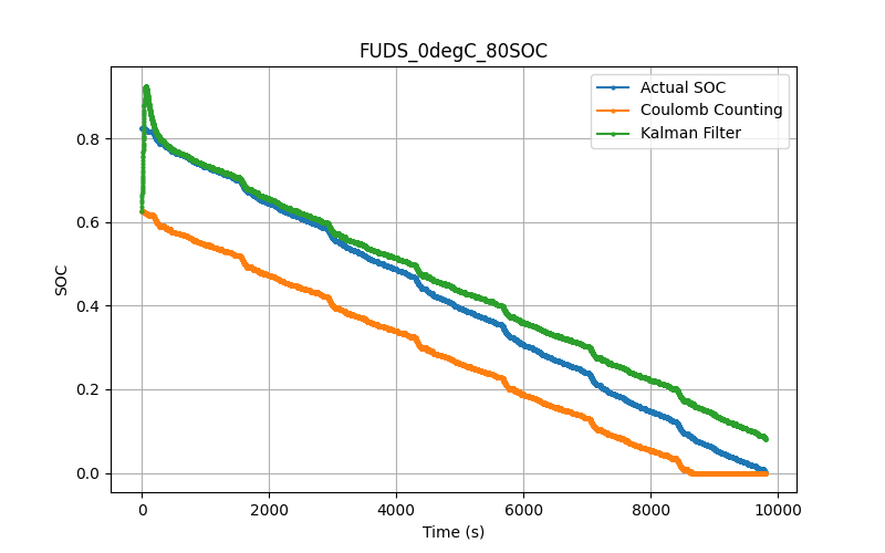
We first look at the SOC results. This is shown on the right were we plot SOC vs time for the Kalman filter, Coulomb counting, and the actual SOC.

We see that the Kalman filter slightly outperforms the Coulomb counting method. In most of the comparisons, we see that the Kalman filter and Coulomb counting methods perform similarly.

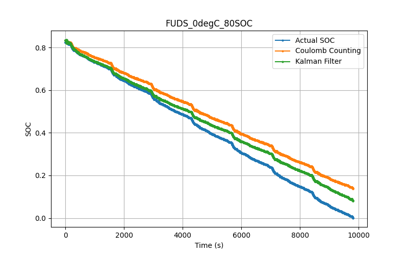
In the results above, it is difficult to say what is the main difference between the Kalman filter and Coulomb counting methods. They give very similar results with similar shapes. In some ways, they almost seem to be offset from each other.

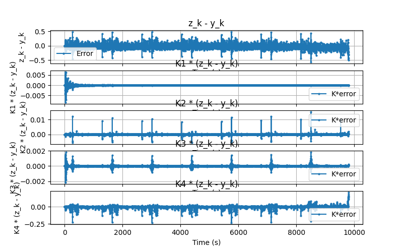
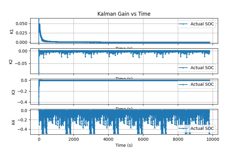
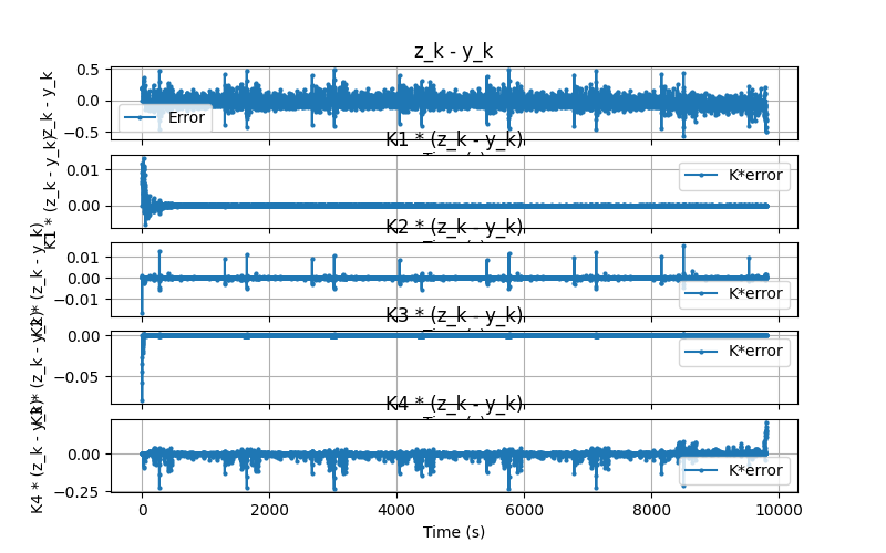
To the right we plot the Kalman gain the Kalman gain multiplied by the difference from measurement and expected measurment. The Kalman gain shows the Kalman gain for each state as a function of time. We see relatively high gains at t=0 but then the gains start to approach zero except for K4 which corresponds to \(V_0\) which we expected. This is expected since \((V_0)_k = i_{k}R_0\), not \((V_0)_k = i_{k-1}R_0\).

The next plot shows the Kalman gain multiplied by the difference from measurement and expected measurment. The first subplot is just the measurement subtracted by the expected measurement to give a sense of magnitude for the correction step. Here we see that the SOC state is barely corrected at all, only about 0.005 at the beginning. We could integrate this correction over time to get a sense of its total impact but I haven't done that yet. However, we know that for this example, the Kalman filter pushed the estimate closer to the actual. It didn't always do that.

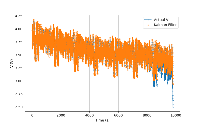
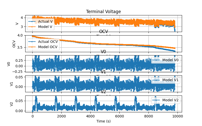
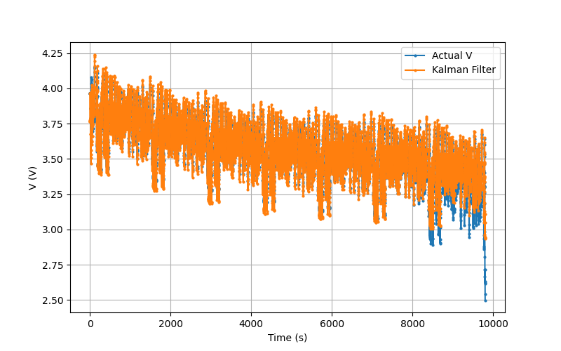
We next compare the voltage estimates to the state voltages (estimated voltages based on the model). This is shown on the right. The first plot (Voltage comparison) shows the terminal voltage (Actual V) and the Kalman filter model voltage. We see fairly good agreement except torwards the end of the test where the SOC is low. This is most likely due to our OCV-SOC relationship/model being relatively poor at low SOC.

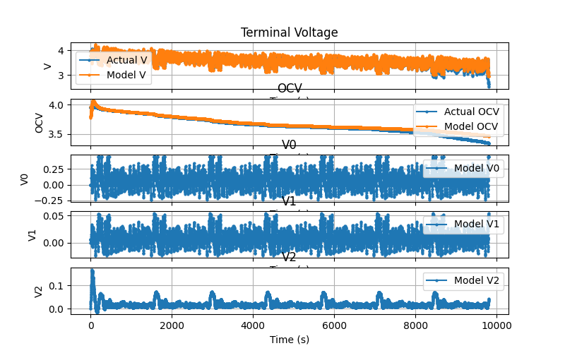
The next plot shows the terminal voltage comparison, OCV voltage comparison (actual OCV is based on the actual SOC), \(V_0\) state, \(V_1\) state, and the \(V_2\) state. For the OCV comparison, we again see pretty good comparison between the actual and the model except at low SOC. This somewhat suggests that our low current test OCV-SOC relationship could be a better fit but I didn't explore this much. We see that \(V_0\) is higher magnitude that the other two RC circuits which isn't too surprising as we do expect some DC resistance across the cell. We see that the two RC circuit voltages, \(V_1\) and \(V_2\), are similar magnitude and vary significantly suggesting this test excites fast and flow dynamics. It's also interesting to note that \(V_0\) and \(V_1\) share a similar shape but are an order of magnitude different.

This test really shows all of the interesting parts of the model and shows some areas we might focus on if we were to improve the model.

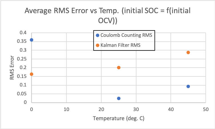
The last plot we have shows the average RMS error comparison between the Kalman filter and Coulomb counting. It is a little surprising that generally Coulomb counting outperforms the Kalman filter. The errors are of similar magnitude and we are assuming the initial SOC for the model is the actual intial SOC. We can imagine in practical applications, that this might not always be true and that we can imagine Coulomb counting deviating from the actual SOC over time due integrating the error.

We'll end this comparison here and in the next section look at the results when the initial SOC is not the actual initial SOC.

In this section, we will show the same results as the previous section but with our initial SOC being 0.75 * the actual initial SOC. This will really show the benefit of the Kalman filter and where it really outperforms the Coulomb counting method.

The SOC estimate results are shown on the right for the scenario where the initial SOC is 0.75 * the actual initial SOC. We see that the Kalman filter almost instantly corrects itself to the actual SOC compared to the Coulomb counting method which has no way of correcting itself.

It's also important to note that the Kalman filter starts to diverge again towards the end of the test similar to how it diverged in the above scenario with the perfect initial SOC. I believe the model to be a little poor and that potentially using an SOC-OCV relationship from the low current test or making the parameters also a function of SOC (or OCV) would improve the model. I would also explore how to tune the process and measurement noises which can influence the Kalman gain (e.g., how much we weight the measurement vs the model).

We now take a look at the Kalman gain and the Kalman gain multiplied by the difference between the measurement and predicted measurement. To really appreciate the differences, we will plot the perfect initial SOC and off initial SOC results side by side below with the perfect initial SOC on the left and non-perfect initial SOC on the right.

The results are very similar for both initial SOC scenarios. We see with the non-perfect initial SOC, that the Kalman correction at the beginning of the test is predominantly in one direction compared to the perfect initial SOC where the Kalman correction bounces around but is centered around 0. This is where the Kalman correction corrects the non-perfect initial SOC. It's cool to see how this small change in the Kalman gain and Kalman correction results in a correction of our SOC estimate.

Next, we will do the same comparison but for the voltages. This is shown below.

Again, the voltage results are very similar between the perfect and non-perfect initial SOC scenarios. We do notice for the OCV voltage vs time in the non-perfect initial SOC scenario, that initially our SOC is low compared to the actual OCV. This is due to us biasing the initial SOC low and we see that the Kalman filter corrects this.

After this initial correction, the results are very similar. It is cool how the Kalman filter can reject this initial disturbance and quickly converges to the actual SOC (even though it starts to diverge a bit after that).

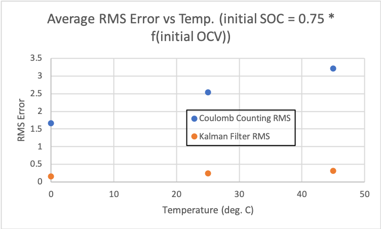
Based on how we see Kalman filter correct itself while the Coulomb counting method does not, it should not be too surprising that the average RMS error for the Kalman filter is much lower than that of Coulomb counting for the scenario with the non-perfect initial SOC. This is shown on the right.

One could argue that the initial SOC being 0.75 * the actual initial SOC is unrealistic but the point is that over time, without being able to correct itself, the Coulomb counting method error will integrate over time and continue to grow. The Coulomb counting method could be improved to include some sort of correction but this is also what the Kalman filter is. We can also modify the Kalman filter to only update every so many time steps. In any case, we see that for this scenario with the non-perfect initial SOC, we have the Coulomb counting RMS error an order of magnitude higher than the Kalman filter error.

It's actually interesting to note that the Kalman filter RMS error for the non-perfect initial SOC scenario is similar to the perfect initial SOC scenario. We show below a comparison of RMS error for each method: Coulomb counting and the Kalman filter.

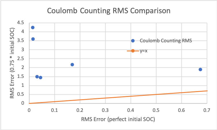
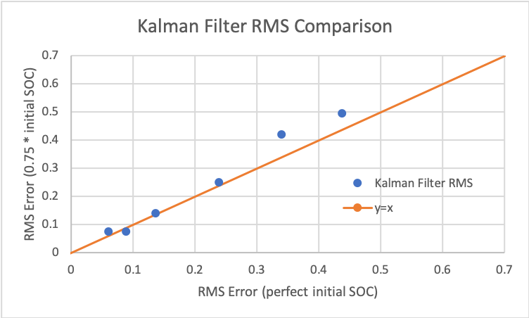
The way to read the plots is that on the y-axis is the RMS error for the non-perfect initial SOC scenario and on the x-axis is the RMS error for the perfect initial SOC. The y=x line is shown to help compare the values. So points above the y-axis correspond to simulations where the RMS error for the non-perfect initial SOC is worse (higher) than the RMS error for the perfect initial SOC. And it's the opposite for when the points are below the y=x line.

We see that the points for the Coulomb counting method are all above the y=x line showing how RMS error is higher for the scenario with the non-perfect initial SOC. However, for the Kalman filter, all the points are near the y=x line, much closer than the Coulomb counting method. This shows how fast the Kalman filter corrects itself and approaches the error when we assume the initial SOC is the actual initial SOC.

This really highlights the advantage of the Kalman filter. The code shows that the Kalman filter doesn't have to be significantly more computationally expensive than the Coulomb counting method but has an extra layer of robustness that the Coulomb counting method alone doesn't possess. And this happens even with a suboptimal model.

Closing Thoughts

Exploring the Kalman filter was a cool experience and helped me improve my linear algebra skills, appreciate noise and measurement challenges, and also exposed me to probability and statistics (something I hope to explore more soon).

I think one of the big takeaways from the Kalman filter is the importance of having a good model of the system and that special attention should be given to tuning based on data (something I ignored for now). It is easy to get carried away with the modeling but this showed me how important it is to understand the dynamics of the process under study and how to capture them. I think a good example here is how the data was given for different temperatures so it's natural to think temperature is a major driver but I think there's a good argument that paramters should also be a function of OCV (or SOC). Maybe I will explore this one day. Maybe having a physical model of the system would help better define this simpler model.

One of the things that has stuck out to me with control system design is how important it is to have a good model. Modeling is half the battle, sometimes more when it comes to designing a controller (before this setting the correct requirements and objectives is also very, very important - something completely ignored here). This was not surprising but helped reinforce what is really important in engineering challenges like this.